Everything in this article (both the text and the images) was generated or gathered by AI; this very paragraph is the only part I wrote myself. I have never systematically studied optics or photography, so I am in no position to vouch for the accuracy of its content. This is simply a reorganization of material I collected while trying to get into photography recently — take it as light reading, and corrections from professionals are very welcome.
If you only ever stay at the level of camera-gear reviews, it is easy to mistake lens design for a permutation of a few labels: large aperture, ED elements, aspherics, high MTF, high resolving power, creamy bokeh, or cinema-grade breathing suppression. But once you truly venture into the world of optical design, you discover that a lens is never the triumph of a single metric — it is a delicate redistribution of an error budget.
A lens’s core mission is utterly pure: to map points in object space onto points on the sensor as accurately as possible. Yet the real world does not permit perfect point-to-point imaging. Rays have angles of incidence, glass has dispersion, surfaces have curvature, and the stop truncates the light bundle; the sensor, too, is not a passive piece of film that merely receives light, but a digital system integrating microlenses, a color-filter array, readout noise, and an ISP. And so “lens design” evolves into an extraordinarily complex problem of holistic optimization: under finite constraints on volume, weight, materials, manufacturing precision, and cost, do everything possible to make enough light arrive, in a sufficiently correct manner, at a sufficiently accurate location.
This article fuses two in-depth research reports into a single accessible beginner’s course: first we build up the basic language of geometrical optics and aberrations, then explore the structural reasons behind the classic lens groups, then analyze the roles of modern materials, aspherics, floating focus, short flange distance, MTF, and computational optics, and finally tie everything together through real-world examples of historical and modern classic lenses.
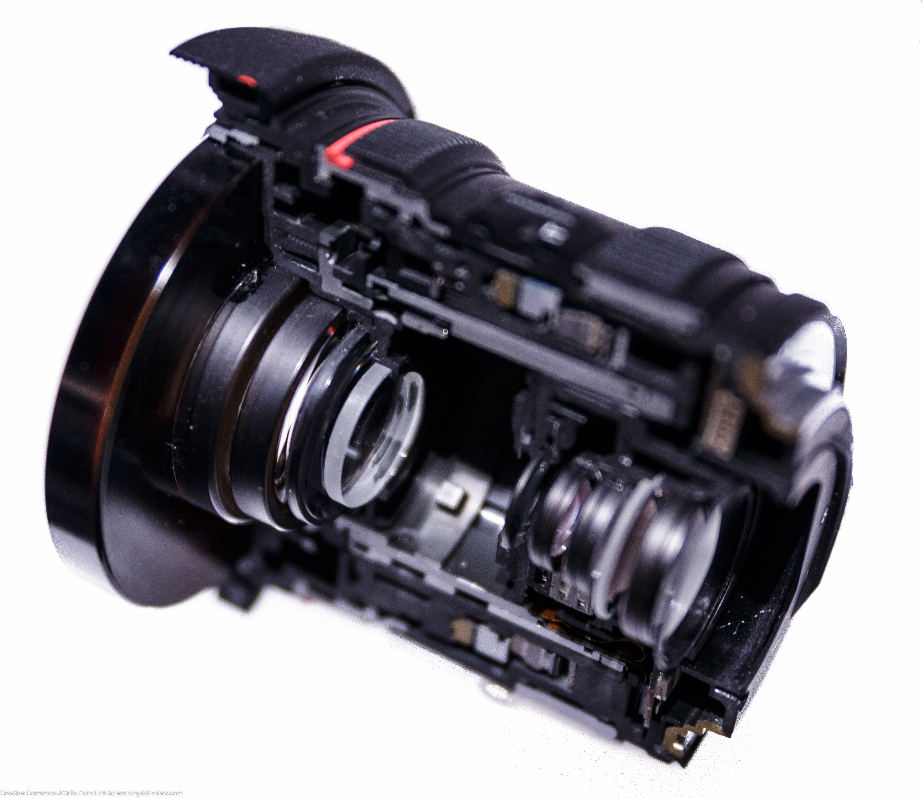
Figure 1: A real lens cutaway illustrates one thing better than any abstract diagram: a photographic lens is not “a few pieces of glass,” but an opto-mechanical system made up of glass, air gaps, the stop, mechanical supports, and tolerances all working together. Source: Wikimedia Commons, Canon L Series Lens Cutaway View, Dave Dugdale, CC BY-SA 2.0.
Before Memorizing Jargon: Picture a Lens as a “Light-Traffic Dispatch System”
When getting started with lens design, what most often trips people up is not the complex mathematics, but the lack of an intuitive mental picture. When you face a pile of seemingly disconnected terms — the stop, the entrance pupil, the chief ray, Petzval sum, MTF, image-space telecentricity — it is easy to feel lost. Rather than rote memorization, it is better to first regard the lens as a light-traffic dispatch system.
Every point on an object radiates a bundle of light in all directions. The lens’s job is to select a portion of that bundle, guide it through the glass and the stop, and finally reconverge it on the sensor into a spot that is as small and stable as possible. Ideally, one object point corresponds to one image point; but in reality, one object point corresponds to a little blob of light, and this blob is called the point spread function (PSF). The better the lens design, the smaller, rounder, and less distorted this blob remains as it moves across the frame.
So you can begin by anchoring three core planes in your mind.
The object plane: where the real world is, how far the object distance is, how wide the field of view is. Photographing the night sky, a portrait, or a microscope specimen means, fundamentally, facing entirely different object-side conditions.
The stop plane: how much light is allowed through, and which marginal rays must be truncated. The aperture does far more than control exposure; it also determines depth of field, diffraction, vignetting, the shape of out-of-focus blur, and the severity of aberrations.
The image plane: where the sensor is, how large the image circle is, and at what angles the marginal rays strike the pixels. In the film era, it was enough for light simply to land on the film; in the digital era, you must also account holistically for the microlenses, the color-filter array, the cover glass, and the in-camera correction algorithms.
The design of all classic lens groups is, at its core, a re-coordination of these three things: planning the path of the light, deciding where to intercept the excess light, and determining the posture with which the light ultimately strikes the sensor. Later, when you study the Cooke Triplet, Tessar, Double Gauss, and Retrofocus, do not rush to count the number of elements. Instead, first ask yourself: Where has it placed positive and negative power? Where is the stop? Which principal plane is it trying to move? Which class of aberration does it most want to suppress?
A One-Sentence Overview: What Is Lens Design Actually Designing?
Lens design is never merely “stacking glass” — it is advancing four engineering efforts at once.
First, establishing the first-order imaging relationships: covering focal length, angle of view, magnification, principal planes, back focal distance, entrance-pupil position, and image-circle size. This determines whether the lens can successfully form an image on the target body and format.
Second, controlling aberrations: including spherical aberration, coma, astigmatism, field curvature, and distortion, plus longitudinal and lateral chromatic aberration. This determines whether the image is sharp, whether the edges fall apart, whether star points smear, whether straight lines bend, and whether colors are misaligned.
Third, allocating engineering degrees of freedom: involving glass materials, curvatures, thicknesses, air gaps, stop position, cemented groups, aspherics, floating groups, coatings, motors, stabilization mechanisms, and mechanical tolerances. This determines whether a theoretical design can be turned into a mass-producible commercial product.
Fourth, planning hardware-software cooperation: deciding which errors are handed off to back-end algorithms, such as distortion correction, vignetting compensation, chromatic-aberration correction, diffraction compensation, deconvolution, HDR, multi-frame fusion, and learned reconstruction. The modern lens is no longer isolated hardware, but one link in the entire “lens-sensor-algorithm” imaging chain.
So, when evaluating a lens, do not merely ask “is it sharp?” The more valuable questions are:
- What optical skeleton did it choose?
- Which aberrations did it prioritize suppressing?
- Which problems did it leave to materials, mechanics, or software to solve?
- What sacrifices did it make for the sake of volume, weight, price, and focusing experience?
1. From the Paraxial Ideal to Real Rays: Where Aberrations Come From
The ideal imaging model is usually built on the foundation of paraxial optics: assume all rays hug the optical axis and have very small angles of incidence, so the sine function can be approximated by the angle itself:
This approximation makes concepts like the thin-lens equation, focal length, principal planes, and magnification easy to compute and handle. Yet modern photographic lenses routinely break this premise: large apertures make marginal-ray angles larger, wide-angle designs make off-axis-ray angles larger, and high-megapixel sensors mercilessly magnify even the tiniest error.
When the angle of incidence is no longer small, we must retain the higher-order terms of the Taylor expansion:
These higher-order terms, ignored by paraxial theory, are precisely the entry point into third-order aberration theory. In other words, aberrations are not manufacturing flaws that arise because “the elements weren’t ground well enough,” but the natural consequence of the simple paraxial model being unable to fully describe the real process of refraction. Manufacturing errors certainly worsen aberrations, but even with flawless workmanship, spherical glass, large ray angles, and a wide field of view are by themselves enough to give rise to all sorts of deviations.
The Thin-Lens Equation Is Concise Enough, but It Only Sketches the “Skeleton”
Introductory study usually starts from the thin-lens equation:
where is the focal length, is the object distance, and is the image distance. This equation conveys a basic principle: when the object is very far from the lens, the image distance approaches the focal length asymptotically; when the object is close, the image distance lengthens. Therefore, when a lens focuses, it must change the relative position between the lens groups and the sensor.
Magnification can be expressed as:
The negative sign represents the image being flipped top-to-bottom and left-to-right. In ordinary photography, the object distance is far greater than the image distance, so magnification is small; but in macro photography, the object distance shrinks dramatically, magnification rises accordingly, and controlling close-up aberrations becomes far trickier. This is exactly why many macro lenses and high-end wide-angle lenses adopt “floating focus”: they do not simply push the whole group forward, but dynamically adjust the spacing of the internal groups at different object distances.
However, the thin-lens equation can only solve the “first-order imaging” problem for you: whether an image forms, roughly what the focal length is, and where the image lands. It cannot tell you whether the edge image quality is sharp, whether blue and red light converge to the same point, and still less can it predict whether the bokeh is beautiful. A real lens is made of thick lenses and multiple groups, and the principal plane may fall inside an element or float outside it entirely. Many of the differences between telephoto and retrofocus structures are, in essence, just a game of “moving the principal plane.”
A beginner can first sort out the differences among these three concepts:
| Concept | The question it answers | Common misconception |
|---|---|---|
| Focal length | Roughly what the field of view and magnification are | Equating focal length with the lens’s physical length |
| Back focal distance | Whether the space from the last element to the image plane is sufficient | Confusing it with focal length |
| Principal plane | Where the equivalent thin lens should be placed | Assuming the principal plane must lie at the exact center of the elements |
The reason the retrofocus wide-angle structure is so great is that it lets a short-focal-length lens have a long back focal distance; the reason a telephoto lens can shorten its barrel is that it makes the effective focal length longer than the lens’s physical length. They look like utterly different lens types, but their core means are one and the same: manipulating the position of the principal plane.
Aperture, the Entrance Pupil, and “Why Does One Stop Faster Cost So Much More?”
The most common — and most commonly misunderstood — formula in photography is the f-number:
where is the f-number, is the focal length, and is the entrance-pupil diameter. Note carefully that this is not the filter thread size, nor the physical diameter of the front element, but the optically effective aperture as seen looking in from the object side.
Take a 50 mm lens as an example:
| Spec | Entrance-pupil diameter | Relative light-gathering area |
|---|---|---|
| 50 mm f/1.8 | 27.8 mm | 1.00 |
| 50 mm f/1.4 | 35.7 mm | 1.65 |
| 50 mm f/1.2 | 41.7 mm | 2.25 |
Going from f/1.8 to f/1.4, the f-number value looks only slightly larger, yet the entrance-pupil area increases by about 65%. And that does not even count the price paid for coping with falloff in edge illumination, vignetting, mechanical obstruction, autofocus-motor load, hood size, and far more demanding tolerance control. So “a faster lens is more expensive and heavier” is by no means an arbitrary manufacturer markup — it is the inevitable result of geometric area, aberration-control difficulty, and manufacturing barriers all soaring at once.
What makes it even thornier is that a large aperture brings not merely “more light gathered”; it simultaneously changes performance across four dimensions:
First, marginal rays increase significantly. Marginal rays most readily expose spherical aberration, coma, and astigmatism. So a lens being sharp at f/4 by no means implies it can easily pull that off wide open.
Second, depth of field becomes extremely shallow. Even the tiniest deviation in front of or behind the focal point becomes impossible to hide. Autofocus error, focus shift, field curvature, and even the photographer’s slight breathing sway will all be magnified.
Third, the rendering of out-of-focus areas becomes crucial. A large aperture makes background blur stronger, but “strong blur” is absolutely not the same as “beautiful bokeh.” Whether the edges of out-of-focus blur disks are harsh, whether onion-ring artifacts are present, and whether edge blur disks turn into cat’s-eye shapes due to vignetting — all of these profoundly affect the overall look of the image.
Fourth, the mechanical burden surges. A larger front group and focusing group mean higher demands on motor thrust; and if you must also satisfy quiet, fast, breathing-free focusing for video, then the optical design and the electronic control system must be deeply co-optimized.
In addition, we must squarely face the physical limit of diffraction. Stopping down can indeed block the “bad rays” at the edge, thereby reducing geometric aberrations, but stopping down too far makes diffraction prominent. The approximate formula for the diameter of the Airy disk is:
Assuming a wavelength of (green light), at f/1.4 we get , while at f/8 we get . This does not mean image quality at f/8 is necessarily worse than at f/1.4, because geometric aberrations are usually more destructive wide open; it merely shows that “stopping down” is not a free, cure-all way to improve image quality, but a search for a new balance point between “reducing geometric aberrations” and “increasing the influence of diffraction.”
In real-world shooting, we often encounter this rule of thumb: many lenses show obvious aberrations wide open and become extremely sharp after stopping down one or two stops; but if you keep stopping down to f/11 or f/16, image quality on a high-megapixel body actually starts to soften. The reason holds no mystery at all — it is precisely because the descending curve of geometric aberrations and the rising curve of diffraction cross over at that point.

Figure 2: The geometric definition of the f-number. The diameter here should be understood as “the effective aperture as seen looking in from the object side,” not simply equated with the filter thread size. Source: Wikimedia Commons, Focal ratio, Vargklo, Public domain.

Figure 3: An intuitive comparison of aperture stops. Each stop down roughly halves the light-gathering area; each stop up roughly doubles it. Source: Wikimedia Commons, Aperture diagram, Cbuckley / Dicklyon, CC BY-SA 3.0.
2. Aberrations: The Lens’s True “Nemesis”
Seidel aberration theory systematically classifies monochromatic geometric aberrations into five types: spherical aberration, coma, astigmatism, field curvature, and distortion. If we add longitudinal and lateral chromatic aberration caused by material dispersion, then the main challenges a photographic lens faces acquire a standard language we can discuss.
| Aberration | Physical mechanism | Image appearance | Common remedies |
|---|---|---|---|
| Spherical aberration | On-axis marginal rays and paraxial rays focus at different points | Soft central image quality, hazy focus, abnormal blur-disk edges | Stop down, use aspherics, balance curvatures |
| Coma | Off-axis bundle loses axial symmetry | Point sources sprout tails; star points at the edge resemble little wings | Symmetric structure, aspherics, optimized stop position |
| Astigmatism | Sagittal and meridional focal points differ | Directional blur in edge lines; a stretching feel in the bokeh | Symmetric structure, joint optimization of field curvature and astigmatism |
| Field curvature | The best focal surface is not a plane, but a curved bowl-shaped surface | The center is sharp while the edges are out of focus, or vice versa | Petzval-sum control, negative groups, floating focus |
| Distortion | Magnification varies with field of view | Barrel, pincushion, or mustache deformation | Optical balancing, software geometric correction |
| Longitudinal chromatic aberration | Light of different wavelengths focuses at different points along the axis | Purple or green fringing in front of/behind focus, especially obvious wide open | Use ED/UD/fluorite materials, apochromatic design |
| Lateral chromatic aberration | Light of different wavelengths is laterally displaced on the image plane | Red-blue / cyan-purple misalignment at the frame edges | Material combinations, symmetric structure, software correction |
From the standpoint of wave optics, a lens does not perfectly restore a point to a point, but converts it into a point spread function (PSF). The more severe the aberration, the more the PSF spreads out, becomes asymmetric, and distorts as the field of view changes. The MTF curve, bokeh texture, sunstar shape, flare control, and edge sharpness are all, at their core, intimately tied to “what shape this point gets smeared into.”
If the table above still seems somewhat abstract, it helps to map each aberration to a concrete photographic problem:
Spherical aberration most readily reveals itself in the central image quality of fast lenses. Ideally, on-axis rays passing through the center and the edge of an element should converge at the same point; but when spherical aberration is present, the marginal-ray focus and the paraxial focus separate along the axis. This means that no matter how you focus, the focal point always carries a hazy “soft-focus feel.” Stopping down can block some of the marginal rays, so spherical aberration usually improves markedly as you stop down. The most direct reason aspherics are irreplaceable is that they can forcibly make these marginal rays “behave.”
Coma is the fatal weakness of astrophotography. The star points at the center of the frame may be perfectly round, but the closer to the corners, the more readily star points turn into little triangles, little bird’s wings, or sprout long tails — usually because the symmetry of the off-axis bundle has been broken. Coma not only makes the edges look “unsharp,” it stretches point sources into directional shapes, severely affecting the look when shooting night-scene lights, the night sky, or stage spotlights.
Astigmatism can be understood colloquially as the lens being unable to “focus simultaneously” in two mutually perpendicular directions. For the same edge point, the lens’s best focus in the sagittal direction and in the meridional direction do not coincide. The result is that lines in some directions are sharp while lines in another direction are quite blurry; the bokeh may also take on a dizzying stretched feel. When the sagittal and meridional curves in an MTF chart separate severely, it usually hints at this kind of problem.
Field curvature is not merely a matter of the frame edges having “low resolving power”; it is the lens’s best focal surface becoming curved. When you photograph a flat wall, if the center is sharply focused while the corners are blurry, but refocusing on the corners makes them sharp while the center goes out of focus, then field curvature is very likely at work. Ordinary portrait shooting can sometimes tolerate field curvature, because the subject is usually not at the edge and the background needs to be blurred anyway; but in architecture, reproduction, astrophotography, and landscape photography, a flat image field is a hard requirement.
Distortion is relatively special: it does not necessarily make the image blurry, but rather warps the geometric relationships within the frame. Barrel distortion makes straight lines bulge outward; pincushion distortion makes straight lines pinch inward. Modern lenses increasingly tend to hand part of the distortion off to software for correction, because the computational cost of geometric straightening is low; but this is not free — the correction process stretches and crops the edges, and in extreme cases loses edge texture detail.
Longitudinal (axial) chromatic aberration often haunts high-contrast edges at large apertures: purple in front of focus, green behind it, or colored halos at the edges of metallic reflections. It occurs along the optical axis, so it cannot be perfectly removed by simply shifting the RGB channels. Lateral (transverse) chromatic aberration, by contrast, appears more at the frame edges, manifesting as colors being laterally displaced from one another; this kind of aberration is relatively easy to correct with software.
The core of studying aberration theory is not memorizing terms, but building the ability to “trace a photographic flaw back to a design pain point.” Seeing “smeared star points,” you should be able to associate it with coma and astigmatism; seeing “the edges just won’t come into focus when shooting a flat plane,” you should realize this is field curvature; “the focal point cloaked in a soft haze” wide open is the signature of spherical aberration and axial chromatic aberration; and “straight lines bending while detail stays sharp” indicates distortion and a lens that relies on software correction.

Figure 4: The crux of spherical aberration is that, for the same color and the same on-axis object point, rays at different heights cannot converge to a single point. Source: Wikimedia Commons, Spherical aberration, Pko, Public domain.

Figure 5: Under ordinary normal dispersion, blue light refracts more strongly and focuses nearer; red light refracts more weakly and focuses farther. Source: Wikimedia Commons, Chromatic aberration lens diagram, Bob Mellish / DrBob, CC BY-SA 3.0.
Chromatic Aberration and the Secondary Spectrum: Why Do Telephoto Lenses Depend So Heavily on Special Glass?
A conventional achromatic group usually strives to bring two wavelength lines (say, red and blue) to converge on the same focal plane as closely as possible. But visible light has more than two lines, and the other wavelengths between red and blue still retain a focusing error. This residual chromatic aberration is called the secondary spectrum.
A material’s dispersion characteristics are usually described by the Abbe number and partial dispersion. The relative partial dispersion can be expressed as:
where and are the refractive indices at specific wavelengths, and and usually represent the refractive indices at the standard blue and red spectral lines. The partial dispersion of most ordinary glasses follows a roughly normal linear relationship with the Abbe number; the expense and value of special materials like ED, UD, Super ED, and fluorite lie precisely in their deviation from this normal straight line, which grants the optical designer an extremely precious “extra degree of freedom for color correction.”
This also explains why telephoto lenses are so ravenously hungry for low-dispersion materials. The longer the focal length, the more severely axial chromatic aberration is magnified; when ordinary glass combinations can do nothing, the designer can only resort to anomalous-partial-dispersion materials, fluorite, diffractive elements, or rely on an even more bloated multi-group design to compensate.
For beginners, here is a very vivid analogy: an ordinary achromatic design is like making red and blue light “shake hands successfully,” but green, violet, and deep-red light may still be standing in different positions. An apochromatic (APO) design, by contrast, aims to act on more wavelengths simultaneously, pinning all the colors to the same point. The reason purple fringing on telephoto lenses is so annoying is that the long focal length magnifies the physical separation of the color foci; and high-megapixel sensors make this separation visible to the naked eye.
This is also exactly why the various manufacturers give their low-dispersion materials a dazzling array of names. ED, UD, Super UD, fluorite, SR, BR, PF, and DO are by no means mere “tier labels” stuck on the barrel; they are distinct weapons developed to solve the problem of color convergence under different wavebands, different physical structures, and different volume constraints. For example, a diffractive element (such as DO/PF) has a dispersion direction completely opposite to that of a traditional refractive element; cleverly exploiting this can effectively cancel chromatic aberration and dramatically shorten the length of a telephoto lens. But at the same time, diffractive elements bring new imaging-style problems such as stray light and ring-shaped flare.
3. Classic Lens Groups: Not Fixed Recipes but Design Priors
When we talk about the Cooke Triplet, the Tessar, the Double Gauss, the Sonnar, the Telephoto, or the Retrofocus, we should not regard them as rigid “element recipes.” They are more like a set of precious “design priors”: telling you in advance roughly how power should be distributed, where the stop is best placed, how the principal planes and back focal distance will move, which aberrations are naturally easy to cancel, and what costs this structure inevitably entails.
Modern commercial lenses continually evolve on top of these classic skeletons: splitting elements, adding cemented groups, swapping in high-index glass, introducing aspherics, piling on ED/fluorite materials, designing complex focusing-group motion trajectories, and even deliberately retaining some residual spherical aberration to shape a particular bokeh texture. The skeleton is merely the starting point of optimization, not its endpoint.
When reading a classic structural diagram, the advice is to drop the habit of “counting elements” and instead examine it with these five questions in mind:
First, how are the positive and negative elements arranged? Positive elements are responsible for converging light, while negative elements are often used to correct field curvature, move the principal plane, or extend the back focal distance. The positional combination of positive and negative elements sets the basic temperament of the lens.
Second, where is the stop? Whether the stop is placed forward, rearward, or centrally directly affects coma, distortion, vignetting, and the positions of the entrance and exit pupils. Many symmetric structures perform excellently precisely because they rely on lens groups that are approximately mirror images in front of and behind the stop to mutually cancel the odd-order aberrations.
Third, where is the cemented group? A cemented group can effectively reduce air-glass interfaces, raising transmittance and contrast, while also exploiting the refractive-index difference between materials to handle chromatic aberration and field curvature. But a cemented group is not an all-powerful “achromatic patch”; its effect depends on the ray height and the material pairing within the system.
Fourth, where has the principal plane been pushed? When studying telephoto and retrofocus structures, what most deserves attention is not the shape of the elements, but where the principal plane and back focal distance have been moved.
Fifth, what shooting goal does this structure serve? Portraiture, a standard kit lens, an SLR ultra-wide, professional sports telephoto, or machine vision? When the target application differs, the very definition of a “good lens” differs completely.
3.1 Petzval: The Mathematical Pioneer of the Fast Portrait Lens
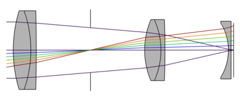
Figure 6: A simplified ray-path diagram of the Petzval lens. The front and rear groups and the central stop together serve fast central portraiture, rather than the full-frame balance of a modern flat-field lens; the edge field curvature and swirly bokeh thus become its signature flavor. Source: Filmmakers Academy, What Does a Petzval Lens Do?.
The Petzval portrait lens is usually regarded as an important milestone in photographic lenses moving from empirical fumbling toward mathematical calculation. Its design goal was extremely clear: in an era when early light-sensitive materials were extraordinarily insensitive, a larger relative aperture had to be used to shorten exposure times, so that portrait photography could become truly commercially viable.
The Petzval’s success stemmed from two things. First, it used multiple groups to separate the tasks of converging power and correcting aberrations — tasks that a single element could not handle simultaneously. Second, it made a decisive trade-off: prioritizing central image quality and maximal light-gathering, while completely abandoning what we today would call “full-frame field flatness.” This trade-off also left an extremely distinct mark: severe edge field curvature and obvious aberrations, with a strong swirling sensation and retro charm at the frame edges.
The lesson this kind of historical lens offers modern readers is: lens design has never been about “eliminating every defect,” but about first defining the purpose. The Petzval was born for portraiture, so central sharpness, light-gathering efficiency, and bokeh atmosphere had the highest priority; edge flatness was simply not on its scorecard.
If you use the Petzval as an introductory case, you will immediately grasp the concept of the “objective function.” The pain point of early photography was not a low corner-MTF benchmark score, but exposure times so long that the subject could not hold still. The Petzval solved the pain point of fast imaging first; as for edge field curvature and swirly bokeh, they were simply not problems at the time. Judging it by modern standards today, we might feel it is “not perfect enough”; but in its own era and given the goals it set, it was an extraordinarily great engineering decision.
This also helps in understanding the review logic of modern lenses. Many lenses are not technically incapable of reaching a certain metric; rather, after weighing the options, the manufacturer chose not to place it first. A cine lens may be willing to sacrifice a bit of absolute resolving power in exchange for ultimate breathing suppression, smooth manual-focus feel, and consistent color across lenses; a portrait lens may deliberately retain a bit of spherical aberration in exchange for creamier, more melted bokeh; and a phone lens may completely let barrel distortion run wild in exchange for a shorter physical module and higher central image quality.
Representative examples:
- The 1840s Petzval portrait lens: the historical starting point of the fast portrait lens.
- Modern reissue Petzval-style lenses: deliberately retaining field curvature and swirly-bokeh effects, turning a historical defect into a modern aesthetic feature.
3.2 Cooke Triplet: Why the Three-Element Structure Is So Pivotal

Figure 7: The positive-negative-positive three-element structure of the Cooke Triplet. It does not rely on stacking elements, but uses minimal degrees of freedom to establish a framework that can handle multiple classes of aberration at once; in actual designs the stop is usually placed near the middle. Source: Wikimedia Commons, Taylor US568052A (Cooke Triplet, 1893 Fig 11), Mliu92, CC BY-SA 4.0.
.svg)
The classic form of the Cooke Triplet is three elements in three groups: positive, negative, positive. It looks extremely crude, yet it is one of the most pivotal turning points in the history of lens design. The reason is that three elements happen to grant the designer just enough degrees of freedom to simultaneously address and balance the various major conflicts among the primary aberrations.
The role of that middle negative element is the finishing touch. To flatten the image surface, the Petzval sum must be controlled, and a negative element happens to provide the opposite contribution. But a simple positive-negative pairing would introduce serious asymmetry problems; so the designer, Taylor, split the positive elements to the front and rear sides, making the whole system approximately symmetric about the central stop. This symmetry is naturally favorable for canceling coma, distortion, and lateral chromatic aberration.
Its advantages are very few elements, low cost, easy computation, and strong potential for derivatives; but its drawbacks are equally obvious: the degrees of freedom are still tight, and the moment you try to challenge a large aperture or a wide field of view, the system quickly falls into a “stressed state” — you have just fixed one aberration and another immediately strikes back. The shadow of the three-element structure can be seen in countless entry-level prime lenses, magnifying lenses, projection lenses, and early camera lenses.
You can understand the triplet as a “minimum-viable aberration-balancing test bench.” The first positive element is mainly responsible for doing its best to gather light, but inevitably introduces spherical aberration, coma, and field curvature; the middle negative element provides opposite power, working hard to flatten the image surface and absorb some aberrations; and the final positive element is responsible for pulling the light back to the final focus while maintaining the balance of the front and rear structure.
Why is it so well suited to study for beginners? Because it reveals the most fundamental trick of lens design: never expect a single piece of glass to be flawless; instead, make different elements introduce errors in opposite directions, then let these errors cancel each other within the system. All the complex lens structures of later generations are, at their core, just frantically adding degrees of freedom on top of this trick: splitting one element into two, upgrading a spherical surface to an aspheric one, replacing ordinary glass with special glass, and turning a fixed air gap into a movable floating group.
Representative examples:
- The Cooke Triplet: the cornerstone of achieving “complete correction with few elements” in modern photographic lenses.
- Countless entry-level camera lenses of the 20th century: trading very few elements for cost advantage, reliability, and ease of mass production.
3.3 Tessar: The Efficient Evolution of Four Elements in Three Groups

Figure 8: The four-element, three-group structure of the Tessar. The rear cemented doublet is not just for “achromatism”; more importantly, within a limited element count, it improves zonal field curvature, astigmatism, and edge performance. Source: Wikimedia Commons, Rudolph US721240A (Tessar, 1902), Mliu92, CC BY-SA 4.0.
.svg)
The Tessar is often called the byword for “four elements in three groups”: two independent elements in front, and a cemented doublet at the rear. It can be seen as a power-boosted version of the Cooke Triplet: adding just one element achieves a qualitative leap in edge image quality and structural efficiency.
Many people mistakenly believe the Tessar’s rear cemented group is merely for eliminating chromatic aberration — this understanding is too one-sided. In a typical Tessar structure, the more critical value of the rear cemented group lies in correcting zonal field curvature, astigmatism, and zonal spherical aberration, which makes its edge performance flatter and sharper than a triplet when covering a larger field of view. It is precisely this extremely high design efficiency that let the Tessar shine throughout the entire 20th century: few elements, high contrast, compact size, and relatively forgiving manufacturing tolerances.
Of course, the Tessar’s shortcoming is its limited large-aperture potential. It can easily produce excellent f/2.8 and f/3.5 standard lenses; but if you try to forcibly scale the heights of large apertures like f/2 or f/1.4, the Tessar’s degrees of freedom fall short, and at that point the Double Gauss structure becomes the more natural choice.
The core of studying the Tessar is by no means rote-memorizing the number “4 elements, 3 groups,” but appreciating the designer’s careful budgeting of degrees of freedom. Adding just one element transformed the structure from the triplet’s “barely all-around” into a “highly efficient tool” for practical photography. The rear cemented group lets the designer handle edge field curvature and astigmatism with a more delicate touch, while the number of air-glass interfaces remains very low. This is why, in an era before coating technology was widespread, the Tessar could still maintain excellent contrast.
This explains why the Tessar became a long-standing favorite as the standard lens for folding cameras and rangefinder cameras. It never chased earth-shattering extreme specs, but bit down hard on the pragmatic bottom line of “sharp enough, small enough, cheap enough, reliable enough.” For an engineer just getting started, the Tessar is a superb case for understanding what makes a good product: a truly high-level design is not necessarily one that piles on materials, but one that trades very few degrees of freedom for a very high degree of completion.
Representative examples:
- Zeiss Tessar 50mm f/3.5 / f/2.8: an industry benchmark for compactness, high contrast, and a minimal element count.
- Countless standard lenses for folding cameras and rangefinder cameras: the Tessar’s unrivaled volume advantage was naturally suited to portable systems.
3.4 Double Gauss / Planar: The Ruler of Fast Standard Lenses
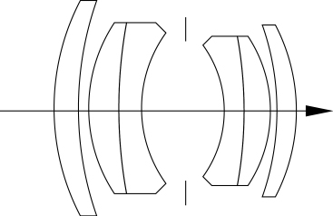
Figure 9: The key to the Double Gauss / Planar is not rote-memorizing “six elements,” but the near-symmetric positive-negative combination around the central stop. This symmetry gives fast standard lenses an excellent starting point for canceling aberrations. Source: Wikimedia Commons, Double-Gauss, Eastwind41, Public domain.
The core soul of the Double Gauss structure is by no means “exactly six elements,” but the near-symmetric distribution of power around the stop. Conceptually, it is usually abstracted as: one side composed of a positive element and a negative meniscus element, with a mirror-like, similar combination placed on the other side. This symmetry gives it an innate advantage in canceling distortion, coma, and lateral chromatic aberration; meanwhile, the addition of the negative groups greatly aids the correction of field curvature and spherical aberration.
This characteristic perfectly fits the demanding requirements of the standard lens. Standard or portrait primes of 50 mm, 55 mm, 58 mm, and even 85 mm must pursue an astonishing large aperture while absolutely not letting distortion and off-axis aberrations spin out of control. The Double Gauss provides a nearly perfect optimization starting point, and precisely for this reason, from the classic Zeiss Planar to everyone’s dazzling array of 50/1.4, 50/1.8, and 85/1.4, the Double Gauss lineage has long monopolized the throne of fast standard lenses.
However, the Double Gauss is not an omniscient answer. When the aperture is pushed further, edge coma, axial chromatic aberration, the harsh edges of out-of-focus blur disks, and field curvature at close focus all charge in like beasts. Modern high-end Double Gauss structures are usually thoroughly “modded”: the groups are stretched and split, and aspherics and low-dispersion glass are introduced in quantity; on a structural diagram they may already look utterly unrecognizable, but the symmetric bloodline still flows underneath.
The Double Gauss is the best teaching material for understanding “the power of symmetry.” Many off-axis aberrations have a clear directionality: when light passes through the front half of the stop it produces an error in one direction, and when it passes through the near-mirror-image structure of the rear half it produces an error in the opposite direction. Although the two can never cancel perfectly in practice, this is enough to press the problem down into a numerical region that is relatively easy to optimize.
A beginner can also use the Double Gauss structure to understand “why sharpness and bokeh are so often at odds.” If the designer pours all their effort into wiping spherical aberration spotlessly clean, the in-focus point image will certainly be razor-sharp, but the edges of out-of-focus blur disks will often become harsh and jarring (the bright-double-line look); conversely, if a bit of spherical aberration is deliberately retained, the bokeh transitions become silky smooth, but the focal point wide open inevitably carries a touch of soft haze. The so-called “having both high resolution and beautiful bokeh” of modern high-end lenses is by no means a flimsy marketing slogan, but the fruit of designers balancing — day after day, at the micron level — the spherical-aberration distribution, asphere precision, stop shape, vignetting, and coatings.
Representative examples:
- Zeiss Planar: the eternal historical totem of the Double Gauss family.
- The Leica Summicron 50mm, along with everyone’s 50mm f/1.4 / f/1.8: the century-long main line of fast standard lenses.
- Nikon Z 58mm f/0.95 S Noct: this is by no means a simple retro homage, but a brute-force challenge — launched against the limits of large aperture, coma control, and ultimate point imaging — using the short flange distance of the mirrorless system and a vast trove of modern degrees of freedom.
3.5 Sonnar: The Fast-Aperture Route of Reducing Air Interfaces and Pursuing High Contrast

Figure 10: The structural emphasis of the Sonnar f/1.5 is compactness, asymmetry, thick cemented groups, and fewer air-glass interfaces. This made it easier to maintain transmittance and contrast in an era when coatings were still immature. Source: Wikimedia Commons, Bertele US1975678A (Sonnar f1.5, 1932), Mliu92, CC BY-SA 4.0.
.svg)
If the Double Gauss represents the elegance of symmetry, then the Sonnar represents an entirely different way of breaking through to a large aperture. In the early days, the biggest predicament the Double Gauss faced was too many air-glass interfaces; in an era when coating technology was still in its savage infancy, this readily caused internal reflections and ghosting and made the image dim and hazy. The Sonnar took a different path, drastically reducing air interfaces through heavy multi-element cemented groups, and with a compact and highly asymmetric structure, sheer-force achieved both high speed (large aperture) and high contrast.
Of course, its aesthetic preferences and engineering costs are equally distinctive. Because it broke symmetry, the Sonnar is more susceptible to spherical aberration, focus shift, and edge aberrations. Interestingly, some modern reissues or lenses that lean into retro mysticism deliberately retain these “defects” in exchange for extremely soft bokeh and a one-of-a-kind tonal transition.
The Sonnar is very well suited to understanding “how an engineering compromise evolves into an artistic style.” When the development goal is news candids, portrait close-ups, the extreme portability of a rangefinder, and the highest transmittance, the Sonnar’s charm is irresistible; but if the goal is “from center to edge, wide open, reaching the monstrous resolving power of a modern flat-field lens,” then it is absolutely not a rational starting point.
There is also a very real historical context behind the Sonnar: early lenses had no modern multi-layer coatings to shield them. The more air-glass interfaces there are, the harder reflection loss and ghosting become to control. The Double Gauss, though theoretically perfect in structure, faced a severe transmittance challenge under the technological limitations of the time. The Sonnar, by “merging” and eliminating multiple reflective surfaces through cementing, was able to hold the line on transmittance and high contrast. From today’s vantage point, with modern nano-coatings now widespread, this approach may seem no longer so urgent, but in the 1930s it was a commercial advantage that could decide life or death.
It is worth noting that the “focus shift” phenomenon brought about by the asymmetric structure is very much worth dissecting on its own. When spherical aberration is present, rays at different heights converge at different focal points; when you stop down, the “bad rays” at the edge are physically blocked, the distribution of rays participating in imaging changes, and the position of the best focus often shifts back or forth accordingly. The user’s intuitive feeling is: I clearly nailed focus wide open, yet after stopping down a stop, the focus drifted on its own. Modern lenses can forcibly suppress this problem with complex floating-focus groups and high-order aspherics, but a retro Sonnar-style lens may treat it as a stubborn bit of character and retain it.
Representative examples:
- Zeiss Sonnar 50mm f/1.5: a legendary classic of the fast standard lens.
- Lenses with Sonnar heritage such as the Nikkor 105mm f/2.5: using fewer interfaces and extremely solid contrast, long serving the portrait and medium-telephoto domains.
3.6 Telephoto: The Magic of Making the Barrel Shorter Than the Effective Focal Length

Figure 11: The skeleton of the telephoto structure is a front positive main group plus a rear negative group. The rear negative group pushes the principal plane out in front of the lens, allowing the lens’s physical length to be shorter than the equivalent focal length. Source: Wikimedia Commons, Lens telephoto 1, Panther, CC BY-SA 2.5.
The essence of the telephoto structure lies entirely in the manipulation of the principal plane. With an ordinary symmetric or conventional design, the physical length of a long lens would be very close to its focal length, and a 300 mm lens would become as awkward to carry as a long spear. The telephoto structure cleverly places a strong positive group at the front to converge the light, then positions a negative group at the rear. The role of this negative group is to forcibly push the system’s principal plane forward, so that the lens’s physical length can be substantially shorter than its equivalent optical focal length.
The cost of this “space-folding” magic is obvious. A long lens is already extremely sensitive to axial chromatic aberration, and combined with the huge front element that must be adopted to satisfy a large aperture, material costs soar exponentially. To ensure the lightning-fast focusing professional sports journalists need while controlling chromatic aberration, spherical aberration, and weight, modern professional telephoto lenses without exception pile on fluorite and UD/ED glass, and come standard with internal focusing, optical image stabilization, and a lightweight magnesium-alloy or carbon-fiber barrel.
The cognitive entry barrier for telephoto lenses is this: you must understand that “long focal length” and “long lens” are completely different things. Focal length is an equivalent optical parameter representing how the lens maps a particular angle of view onto the sensor; the lens’s physical length is merely the final result of mechanical design.
Why are professional telephoto lenses so expensive? Let’s do the math with a 300mm f/2.8 as an example. Its entrance-pupil diameter is approximately:
This means the effective light-gathering aperture at the front already exceeds 10 centimeters. To make such a huge bundle of light still deliver razor-edge sharpness wide open, the front glass block must be machined to be both enormous and precise; to ensure red, green, and blue light do not part ways after their long journey, extremely expensive fluorite or top-tier UD glass must be deployed; to keep the autofocus motor from being slow and sluggish under an unbearable load, the entire heavy front group must absolutely not participate in the focusing motion, so an internal-focus design driving a light rear group is the only option; and to allow handheld shooting, an extremely precise optical-stabilization module must also be crammed in. This is why professional telephoto lenses look like “artillery pieces” — not for the sake of a flashy look, but as a form forced out by the cruel laws of optical physics.
If you scrutinize the official cross-section of a super-telephoto lens, you will find that the most expensive special glass is almost entirely concentrated in the front-center, while the focusing elements are often the unremarkable small elements in the mid-rear. This is the classic collaboration of optics and mechanics: the largest glass greedily absorbs light and sets the tone of image quality, the light little groups handle lightning-fast focusing, and the suspended stabilization group deflects the light path in real time to resist vibration.
Representative examples:
- The Canon EF 300mm f/2.8L series: the absolute workhorse of professional sports and wildlife photography, the culmination of fluorite/UD materials with internal focusing and stabilization.
- Nikon, Canon, and Sony’s 400mm f/2.8 and 600mm f/4: relying on materials science, precision mechanics, and stabilization algorithms to jointly tame the heavy costs the telephoto structure brings.
3.7 Retrofocus: Why SLR Ultra-Wides Are Destined to Be Large and Complex

Figure 12: Retrofocus is also called inverted telephoto; a large front negative group lengthens the back focal distance, leaving mechanical space for the SLR mirror. The cost is that distortion, corner aberrations, and front-group size all become harder to control. Source: Wikimedia Commons, Angenieux - Retrofocus (1950), Mliu92, CC BY-SA 4.0.
.svg)
The retrofocus structure can be seen as the “reverse operation” of the telephoto structure: a strong negative group is placed at the front of the lens to forcibly diverge the light, after which a rear positive group reconverges it. The historical mission of this design is extremely clear: in SLR camera systems, the mirror occupies a huge mechanical space behind the lens, making it impossible for a wide-angle lens to land its focus extremely close to the last element.
Suppose you want to develop a 20 mm wide-angle lens for an SLR system with a flange distance of over 40 millimeters; if you use an ordinary symmetric wide-angle structure, the rear group would slam right into the mirror. The retrofocus structure perfectly solves this mechanical-interference problem by lengthening the back focal distance. But the price it demands is equally brutal: the front element must be made enormous and bulging outward, barrel distortion runs rampant, and edge aberrations and field curvature are hard to suppress. Precisely for this reason, in the SLR era, high-performance ultra-wide lenses were often synonymous with “big, heavy, expensive, and unable to mount conventional filters.”
To understand the retrofocus structure more intuitively, imagine how the light is forcibly “tortured.” An ordinary 20mm lens could have simply and directly refracted the light onto the sensor quickly, but to make way for the mirror, the designer is forced to use the front negative element to “pull apart” (diverge) the already very wide field of view, then desperately use positive elements to “gather” the light back together in the limited rear space. This operation of diverging first and converging later sheer-force props open a stretch of back-focal-distance space.
However, that strong front negative group inevitably brings exaggerated barrel distortion and makes the marginal rays enter the subsequent groups at extremely steep angles. When you see that bulbous, protruding front element on an SLR ultra-wide lens, it is by no means for the sake of an exaggerated visual impact, but to laboriously catch those obliquely incident rays from a super-wide field, and then, across the dozens of elements that follow, to painstakingly drag distortion, field curvature, astigmatism, and chromatic aberration back onto the right track little by little. The larger the aperture and the wider the angle, the deeper this torment.
With the arrival of the mirrorless era (short flange distance), the survival pressure on the retrofocus structure has been somewhat relieved, but it has not completely died out. The reason is that modern high-megapixel digital sensors deeply detest overly oblique edge chief rays. To control the CRA (chief ray angle), vignetting, and edge aberrations, wide-angle lenses still need to maintain a certain back focal distance. The short flange distance does grant the designer more options, but it absolutely does not mean all ultra-wide lenses can turn into lightweight little “pancakes” overnight.
Representative examples:
- Angenieux Retrofocus 35mm f/2.5: the key pioneer that pushed the retrofocus wide-angle toward practical SLR use.
- Nikon AF-S 14-24mm f/2.8G ED: the legendary holy grail of SLR ultra-wide zooms, relying heavily on the synergy of the retrofocus skeleton, an enormous front group, aspherics, and ED glass.
- Sigma 14mm f/1.8 Art: to achieve the extreme f/1.8 aperture at ultra-wide, it had to resort to an extremely brute-force front-group design and rigorous aberration control.
3.8 Telecentric: Not for Ultimate Sharpness, but for Absolute “Measurability”
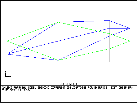
Figure 13: A telecentric lens cares about the posture of the chief ray. Making the object-space or image-space chief ray nearly parallel to the optical axis reduces the problem of magnification varying with distance, which makes it especially suited to measurement and machine vision. Source: Wikimedia Commons, 1 to 1 telecentric 2L paraxial relay lens, JonesMI, Public domain.
The telecentric lens is often misunderstood in photography circles as some kind of “dimension-crushing advanced photographic lens.” In fact, its core pursuit is not the subjective impression of “sharpness” at all, but industrial-grade measurement stability. The core of the telecentric design is that it can force the chief ray to enter or exit almost parallel to the optical axis. As a result, when the object being measured undergoes a slight change in distance along the depth direction, the imaging magnification barely changes at all; in a doubly telecentric design, even a slight mounting error in the sensor position can be immunized against.
This explains why telecentric lenses have all but conquered machine vision, precision dimensional measurement, wafer-defect inspection, and automated production lines, yet rarely appear in ordinary photography. They tend to be bulky, demand a very large aperture, and are costly, but in return they completely eliminate perspective error and magnification drift.
The charm of ordinary photography often comes from perspective relationships (near objects look larger, far objects smaller), whereas the telecentric lens devotes its life to annihilating perspective. If you use an ordinary lens to photograph a round hole, the moment the hole gets a little closer to the lens, it looks larger in the frame; in industrial inspection, if the height of a workpiece surface undulates slightly, the dimensional measurement will suffer a fatal deviation. By ensuring the chief rays are parallel, the telecentric lens keeps the size projected onto the sensor nearly constant as the measured object moves within a certain depth of field, thereby becoming the anchor of precision measurement.
This also explains why the aperture of a telecentric lens often looks “extremely exaggerated.” To keep all the chief rays across the entire field parallel, the entrance aperture of the lens must be greater than or equal to the actual size of the object being measured; it cannot rely on perspective to compress the field of view the way an ordinary wide-angle lens does. It willingly sacrifices portability and low cost solely to obtain that irreplaceable “measurement repeatability.”
Representative examples:
- Industrial telecentric lenses from brands such as Schneider, Edmund, and Thorlabs: widely used in dimensional verification, aperture scanning, and high-precision robotic-arm positioning.
- Wafer-level and panel-level vision-inspection systems: in these domains, telecentricity and field flatness matter ten thousand times more than “whether the bokeh melts away.”
3.9 Zoom: The Abyss of the Zoom Lens Is “Many Conditions Holding Simultaneously”
Figure 14: A highly simplified animation of the zoom principle. A real photographic zoom must also add a compensation group, a focusing group, a rear-correction group, and complex cam tracks, but this image first captures the core of “multiple groups moving relative to one another.” Source: Wikimedia Commons, Zoom prinzip, Smial, CC BY-SA 2.0 DE.
The terrifying complexity of the zoom lens has never lain in the single function of “being able to change focal length,” but in this: throughout the entire dynamic process of changing focal length, the position of the image plane must be locked down tight, and aberrations, distortion, relative edge illumination, the mechanical travel of the motion, and the focusing feel must all be kept within an acceptably high standard.
The total power of an extremely simplified two-group zoom system can be expressed as:
where and are the powers of the two groups respectively, and is the spacing between them. Changing the inter-group spacing changes the total power of the system, which is to say it changes the focal length. But this is merely fairy-tale theory. The design of a real zoom lens is far more irascible than this formula: you must simultaneously control the image plane against drift, keep the entrance-pupil position reasonable, suppress wildly varying distortion and CRA, precisely compute the curve tracks of the mechanical cams, and squeeze a passing MTF score out of every focal length.
Constant-aperture zoom lenses are an even greater nightmare for engineers. A 24-70mm f/2.8 already requires multi-dimensional optimization under a vast number of conditions; if a manufacturer attempts to challenge a 28-70mm f/2, the demand for entrance-pupil area and the pressure of aberration control explode exponentially. The reason such holy-grail lenses are so astonishingly large is precisely that they must maintain professional-grade light-gathering and ultimate image quality at every checkpoint from wide-angle to medium-telephoto.
Designing a prime lens is like deep-mining the optimization at a single point in three-dimensional space; designing a zoom lens is like performing an acrobatic balancing act along an undulating, twisting curve. At the 24mm wide end, you must desperately suppress the strong distortion and vignetting brought by the large field of view; at the 70mm long end, you must turn around and deal with axial chromatic aberration, working hard to improve the resolution and bokeh at the long end; and at all the intermediate focal lengths between these two ends, you must absolutely not leave any “sunken zone” where image quality collapses. What is even more despairing is that the moment the user changes the focusing distance (say, moving in close for macro), all the optimization balance you just built is instantly broken, and everything has to be done over again from scratch.
The essence of mechanically compensated zoom lies in this: the variator group charges into battle to change the focal length, while the compensator group moves in sync like a shadow, its sole mission being to precisely pull the image plane — which has drifted off because of the zooming — back onto the plane of the sensor. This motion is by no means a casual slide, but a micron-level constraint enforced by extremely complex mechanical cam slots or electronically controlled motor tracks. If the compensation track is even slightly flawed, the user will find the focus drifting around when pushing and pulling the zoom ring; if the barrel’s coaxiality control is poor, video creators will see the center of the frame drift laterally; and if the internal-focus compensation algorithm is not clever enough, the angle of view will visibly magnify or shrink while focusing — the “breathing” that the video industry loathes.
So a modern 24-70mm f/2.8 is absolutely not as simple as “crudely splicing together several prime lenses of different focal lengths.” It is the ultimate comprehensive examination of a manufacturer’s capabilities in optical design, precision machining, automatic-control algorithms, weather-sealing technology, quality consistency, and even cost control. Many seemingly unremarkable standard zoom lenses are in fact what best represents an optical giant’s true industrial depth.
Representative examples:
- Angenieux’s early mechanically compensated zoom lenses: turned zoom technology from a laboratory toy into a practical productivity tool for the film and news industries.
- 24-70mm f/2.8: the classic benchmark and touchstone of the professional standard zoom.
- Canon RF 28-70mm f/2L USM: in the mirrorless era, exploiting the huge mount diameter, the extremely short flange distance, and a maniacal pile of optics to forcibly make a constant-f/2 standard zoom a reality.
3.10 Phone Lenses: The Ultimate Deep Binding of Optics and Algorithms
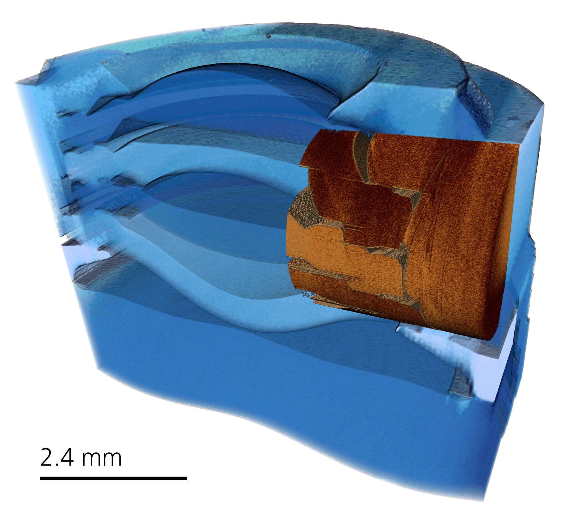
Figure 15: A 3D X-ray micrograph of a smartphone camera module. Even within this tiny module there are still multiple elements, filter structures, supports, and assembly tolerances; the optical design must be considered together with manufacturing and algorithms. Source: Wikimedia Commons, Mobile phone camera lens module, 3D X-ray microscopy, ZEISS Microscopy, CC BY 2.0.
.jpg)
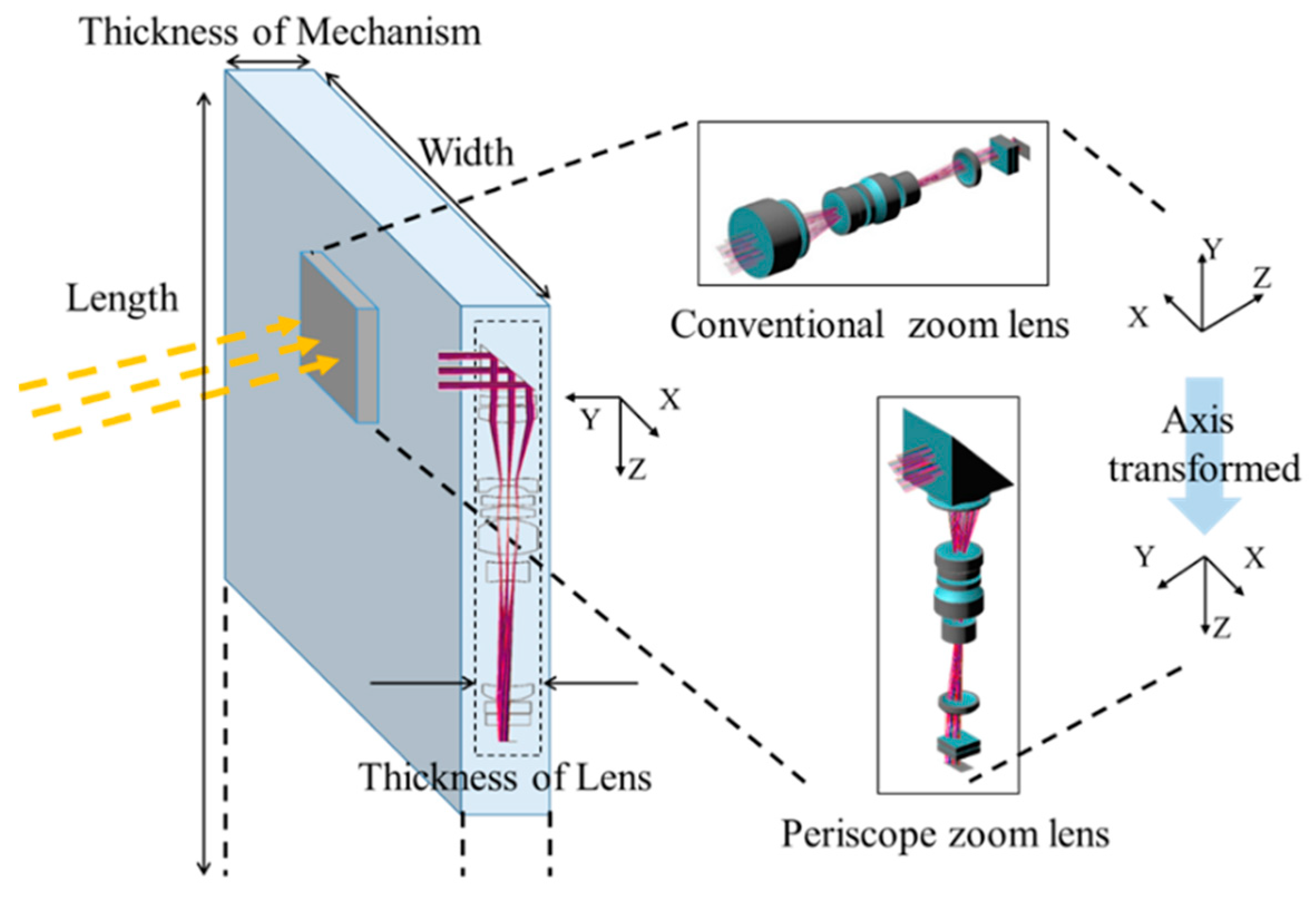
Figure 16: A periscope phone lens folds the light path inside the body, trading lateral space for a longer focal length. It is not the opposite of “algorithmic zoom,” but a typical direction in which phone optics, structure, and algorithms compromise together. Source: Wikimedia Commons, Periscope zoom lens vs conventional zoom lens in a smartphone, Wen-Shing Sun, Yi-Hong Liu and Chuen-Lin Tien, CC BY 4.0.
The smartphone camera represents an extraordinarily extreme school within modern lens design: a small sensor area, extremely small individual pixels, a module thickness held down tight, an extremely short focal length, very large edge incidence angles, large-scale use of plastic aspherics, and deep reliance on the forceful intervention of post-processing algorithms. Traditional photographic lenses usually carry a classical pride — pursuing “as much perfection as possible at the level of pure physical optics”; whereas phone lenses have completely tilted toward “systems-engineering computation”: meticulously calculating which aberrations the plastic elements must endure head-on, which deviations are made up for by shifting the sensor’s microlenses, and then throwing the remaining catastrophes entirely to the powerful ISP (image signal processor) and multi-frame fusion algorithms to “defy fate.”
A simple field-of-view estimate is enough to expose the desperate situation phones face. Suppose the sensor’s horizontal width is and the target horizontal field of view is ; the focal length can be approximated as:
If and , then . If the target aperture is as fast as f/1.8, then the entrance-pupil diameter is about:
This means that, within an extremely cramped microscopic space, large-angle rays must be forcibly bent. If the sensor’s individual pixel size approaches 1 µm, then the conflict among the diffraction limit, optical aberrations, and the sensor’s sampling rate becomes a hair-trigger affair. The diameter of the Airy disk is approximately:
Taking and , we get . This number coldly declares: a phone simply cannot, like an SLR lens, mask aberrations by merely “stopping down,” because the moment the aperture shrinks, diffraction instantly devours all the high-frequency detail. Therefore, the modern phone has no choice but to sprint down a road of no return — paved with extremely high-order aspherics, rigorous CRA (chief ray angle) matching, brute-force digital stretching of geometric distortion, algorithmic vignetting compensation, deep deconvolution, multi-frame stacking and fusion, and ultimately heading toward “end-to-end joint optimization” of the optical prescription and an AI reconstruction network.
Phone lenses also have a life-or-death line that traditional cameras need not face: the total module length. A phone is only a few millimeters thick, and this slim space must not only hold 7 to 8 elements, but also reserve room for the autofocus voice-coil motor, OIS optical stabilization, dust-and-water-resistant structures, the infrared filter, the sapphire cover glass, and the inevitable assembly tolerances. The designer has no luxury of a “long air gap” to slowly tame aberrations, and can only, within a narrow tube of less than a centimeter, rely on stacking many extremely distorted high-order aspheric plastics, or glass-plastic hybrid elements, to forcibly accomplish the refraction and convergence of light in an almost brute-force manner.
This is why a phone lens, though seemingly as small as a bean, hides an engineering complexity that is staggering. Every wafer-thin plastic asphere inside bears an unbearable weight: it must control distortion, flatten field curvature, correct CRA, and bite down hard on the module-thickness limit. The price of this extreme maneuvering is extreme sensitivity to manufacturing tolerances and thermal drift. Therefore, a phone’s imaging output absolutely cannot rely on the optics department alone; it must be a system crystallization jointly calibrated by the optics, structural-module, semiconductor-sensor, and imaging-algorithm teams.
So when you see a photo on a phone whose edge detail may have been forcibly stretched by algorithms, whose vignetting has been digitally brightened, whose noise has been smoothed away across multiple frames and re-sharpened, please do not simply mock it as “software cheating after an optical failure.” A more accurate understanding should be: from the very first day a smartphone was conceived, it never intended to be a pure optical lens. It is a “computational imaging system.” The optics’ job is no longer to deliver a perfect image, but to capture “enough, and mathematically recoverable” raw information; subsequently, the algorithms take over everything, reassembling this information into a beautiful image the human eye is glad to accept.
Representative examples:
- The multi-element plastic/glass hybrid modules of various flagship phones: an extremely short total length, extremely complex aspheric surface shapes, and heavy reliance on software post-correction.
- Cutting-edge academic research represented by DeepLens: completely breaking down the wall between hardware and software, placing the complex refractive-lens parameters and the back-end AI reconstruction neural network within the same differentiable framework for global optimization.
4. The Four Classes of Freedom in Modern Lenses
If classic structures define a lens’s “skeleton,” then modern optical technology determines a lens’s “ceiling.” The reason today’s high-performance lenses are so powerful is, at its core, not simply piling on more elements, but that the designer holds far more “allocatable degrees of freedom” than their predecessors did.
Surface Freedom: Aspherics (Aspherical)
The machining process for spherical lenses is extremely mature and the inspection methods are very well developed, but a spherical surface inherently produces spherical aberration. An aspheric lens breaks the constraint of a single curvature, letting the curvature change continuously with the radial position on the element. Its core value lies in being “worth ten on its own”: using one complex aspheric surface to take on the aberration-correction tasks that previously required a combination of several spherical surfaces.
A common aspheric sag equation can be expressed as:
where is the vertex curvature, is the conic constant, and are the higher-order aspheric coefficients. In optical-design software, this formula looks like a magic wand the designer can wave at will; but the factory’s shop foreman will immediately pour cold water on you: the more the surface deviates from a standard sphere, the harder it is to machine, the more maddening the surface-form inspection becomes, the more the cost soars geometrically, and the more readily microscopic tool marks are left on the surface, ultimately ruining the texture of out-of-focus highlights.
The strategic value of aspherics is mainly reflected in three places:
- Strongly suppressing spherical aberration, coma, and severe distortion.
- Dramatically reducing the element count, making the system lighter and shorter.
- Providing make-or-break key degrees of freedom in ultra-wides, extreme large apertures, large zoom ratios, and extremely constrained phone lenses.
But the price it demands is equally clear:
- It imposes hellish demands on the machining precision of glass molding or precision grinding.
- The microscopic texture of the surface (often coming from machining traces in the mold) casts ugly concentric rings in out-of-focus highlight blur disks, colloquially called “onion rings.”
- If left unconstrained, the design software readily produces bizarre surface forms that are flawless on the mathematical curve but utterly unmanufacturable on the shop floor.
If we put aspherics back into a real lens structure, their role becomes clear at a glance. In fast standard lenses, aspherics are usually used to suppress spherical aberration and coma, ensuring razor-sharpness wide open; in ultra-wide lenses, that huge frontmost asphere is mainly used to subdue barrel distortion, corner astigmatism, and field curvature; the heavy use in zoom lenses is because, to hold image quality steady across different focal lengths, the degrees of freedom of spherical surfaces have long been stretched thin; and in phone lenses, aspherics are even the only lifeline, because the module is so thin that there is no room to slowly correct the light path with multiple large glass elements.
However, aspherics are by no means “the more the better.” If the designer makes a single asphere bear too many correction tasks, its surface-form variation becomes extremely aggressive, which not only sends manufacturing and inspection costs out of control, but also makes mass-production consistency a disaster. The “onion rings” in the bokeh that photography enthusiasts often complain about are, to a large extent, a by-product of this extreme squeezing of asphere machining precision. Therefore, when a high-end lens emphasizes “high-precision aspherics” or “ultimate surface smoothness” in its marketing, this is not only to improve in-focus resolving power, but also to ensure that out-of-focus highlights are not sullied by rough manufacturing traces.
So when you are looking at a lens structure diagram and find ASPH marked on it, please do not merely translate it as “premium configuration.” The more professional question should be: is this asphere placed in the front group where ray height is extremely high, or in the rear group near the sensor? Is its primary task to suppress spherical aberration, coma, and distortion, or merely to reduce element count to control size? If it exists in a fast lens that touts itself for portraiture, we must also sternly scrutinize its negative impact on the texture of out-of-focus highlights.
Material Freedom: ED, Fluorite, and Anomalous Partial Dispersion
The relationship between refractive index and dispersion in ordinary optical glass is confined to a relatively rigid range. To precisely force light of multiple wavelengths onto the same focal plane, especially in the extreme scenarios of long focal lengths and very large apertures, special materials with “anomalous partial dispersion” must be introduced.
The market is flooded with each manufacturer’s dazzling array of abbreviations: Canon’s prized Fluorite, UD, Super UD, BR, and DO; Nikon’s ED, Super ED, SR, and PF; and Sony, Sigma, and Tamron also each have their own named low-dispersion glasses. Please do not simply regard these abbreviations as “tier stickers” distinguishing a lens’s rank; they each correspond to different target wavebands, different forms of aberration pain points, and different volume-weight compromise schemes.
A more fundamental way to understand it is that when the ordinary “crown glass” and “flint glass” combination has exhausted its potential, the designer is left with only three routes of breakthrough:
- Change the material: use ED, UD, and natural or synthetic fluorite regardless of cost, or even develop new high-index, low-dispersion special glasses.
- Change the phase mechanism: introduce diffractive optical elements (DO/PF), exploiting their physical property of a dispersion direction completely opposite to that of traditional refraction to cancel chromatic aberration.
- Change the structure: add more separated groups, thick cemented groups, or forcibly lengthen the entire optical system, trading extremely uneconomical geometric space for the freedom of color correction.
Why do telephoto lenses and fast lenses have an almost pathological dependence on this kind of special material? Because longitudinal chromatic aberration becomes abnormally glaring as the focal length lengthens and the light bundle grows. A 24mm wide-angle lens with a bit of axial chromatic aberration is often masked by the huge depth of field and complex scene detail; but if a 300mm f/2.8 lens shows color-focus separation at a high-contrast edge, the image will instantly erupt into disastrous purple and green fringing. A larger entrance-pupil area lets more unruly marginal rays participate in imaging, which further magnifies “spherochromatism” — the thorny problem of spherical aberration wandering as a function of wavelength.
The reason fluorite is held as the gold standard is that its extremely low dispersion and extraordinarily prominent anomalous-partial-dispersion characteristics have irreplaceable strategic value in telephoto systems; but its drawbacks are equally fatal: high manufacturing cost, extreme fragility during machining, and sensitivity to temperature changes. ED/UD glass, by contrast, is the modern mainstay that strikes a perfect balance between material performance and industrial mass production. As for diffractive elements (such as DO/PF), their approach is even more ingenious: traditional refractive elements usually have a higher refractive index for blue light (stronger refraction at shorter wavelengths), while the dispersion direction of diffractive elements is exactly the opposite; combining the two can not only strongly cancel chromatic aberration but also dramatically shorten the barrel length. But the diffractive structure is by no means a free lunch — it readily brings hard-to-control stray light, jarring ring-shaped flare, and an extremely high microstructure-manufacturing barrier. It is a sharp tool, not a perfect panacea.
When facing a manufacturer’s marketing about materials, one must beware of a common cognitive pitfall: the quantity of special glass absolutely cannot be directly equated with the level of image quality. A lens that piles in three ED elements does not necessarily perform better than one that uses only two. The true deciding factor is: at which nodes in the light path are these expensive materials placed? With what spherical or aspheric curvatures are they paired? Just how large are the target focal length and aperture specs? And does the final overall aberration reach a harmonious balance? Materials are merely chips in the designer’s hand, and having more chips does not guarantee winning in the end.
Electro-Mechanical Freedom: Floating Focus, Internal Focus, Stabilization, and Aperture Actuators
In the traditional era, lens focusing usually relied on the entire optical system moving back and forth as a whole, and when optimizing aberrations, designers often leaned most of their effort toward the “infinity” reference point. However, the drawback of this design is that, the moment you enter close-range shooting, the sharply changing object distance instantly tears apart the painstakingly constructed light-path balance, and spherical aberration, astigmatism, and field curvature may deteriorate avalanche-fashion at close focus.
The solution of floating focus (floating focus / close-range correction system) is this: break the rigid rule of “the whole group moving in and out together,” and let two or even multiple groups inside the lens move relative to one another along entirely different trajectories and speeds during focusing. As a result, whether at infinity or at the macro end, the lens can dynamically adjust in real time to maintain the closest-to-perfect aberration balance. Macro lenses, fast wide-angle lenses, and modern video lenses that pursue demanding breathing control depend heavily on this mechanism.
It brings two immediately apparent benefits:
- It greatly preserves image quality during close-range shooting, avoiding a collapse in resolving power.
- It provides precious room for trajectory optimization to suppress focus breathing, correct focus shift, and control edge aberrations.
But the engineering costs hidden behind this are equally brutal:
- It requires designing and machining extremely complex mechanical cam slots, or equipping multiple independent high-precision electronically controlled motors.
- The decentering, tilt, and tiny mechanical play of each moving group during motion all directly translate into optical disasters.
- The costs of factory assembly and optical-axis alignment rise sharply.
The design logic of stabilization systems (IS/VR/OIS) is of the same lineage as floating focus. Modern in-lens optical stabilization is by no means an “add-on feature” bolted onto the barrel, but suspends one particular compensation group and deflects the light path in real time by moving it at high frequency, thereby canceling hand shake. This amounts to tying extremely sensitive gyroscope sensors, voice-coil-motor actuators, a closed-loop position-feedback system, and the underlying optical design tightly and inseparably together.
We can use an everyday example to understand “floating focus” colloquially: a traditional lens optimized superbly at infinity is like a table sitting on a level floor with its four legs perfectly shimmed; when the focusing distance moves in close, it is like moving this table onto a patch of bumpy, uneven mud. Whole-group focusing is like merely translating the entire table over, and the result is inevitably wobbling and instability (image-quality decline); floating focus, by contrast, is like independently and dynamically adjusting the length of each of the four legs according to the terrain while moving the table, ensuring the tabletop always stays absolutely level (the aberrations are re-shimmed flat).
The significance of internal focus (Internal Focus) goes far beyond the cosmetic elegance of “the lens not extending while focusing.” Its core value lies in driving only a lighter, smaller group inside, thereby greatly boosting autofocus speed, lightening the load on the focusing motor, and avoiding the trouble that front-group rotation causes for polarizers and graduated filters. But because internal focus moves only some elements, this inevitably changes the system’s overall aberrations and effective angle of view, so designers must invest a huge amount of effort to recompute its motion trajectory. The reason many video-lens manufacturers loudly tout their “minimal breathing” is precisely that, if the focusing group’s motion is not intervened upon, it will not only change the focal plane but also change the effective focal length along with it, causing the annoying zoom in the frame.
The aperture actuator likewise profoundly affects the final shooting experience. The electromagnetic diaphragms, linear motors, stepper motors, VCM voice-coil motors, and stabilization actuators integrated inside modern lenses have long become an inseparable part of the complete optical system. Their response speed and precision determine whether the designer’s paper optical prescription can be translated into stable, reliable performance in the harsh field: is the exposure perfectly consistent during high-speed burst shooting? Is the transition of a video focus pull silky smooth? Will the stabilization module’s violent compensation trigger periodic fluctuations in edge image quality? These invisible electro-mechanical performances ultimately become real, tangible experiences in the photographer’s hands.
System Freedom: Short Flange Distance, Sensor Microlens Matching, and Software Computational Correction
With the rise of mirrorless camera systems, the mirror has been thrown thoroughly into the dustbin of history, the flange distance has been greatly shortened, and the last element can even snug right up against the sensor. For wide-angle and standard lenses, this is nothing short of shedding a heavy historical burden: designers no longer have to rack their brains, as in the SLR era, to forcibly lengthen the back focal distance to dodge the mirror. The lens structure can return to a more naturally symmetric form, or boldly adopt rear groups of even more exaggerated diameter, thereby greatly improving the incidence angle of edge rays and raising image-space telecentricity.
However, a digital sensor is by no means flat film. Above the sensor’s silicon substrate are densely packed microlens arrays, the Bayer color-filter array, and a thick low-pass/cover glass. If the lens’s edge chief ray angle (CRA) is tilted too outrageously and does not match the offset design of the sensor’s edge microlenses, it will immediately induce severe edge color shifts (red-green patches), vignetting, and a collapse in frame uniformity. Therefore, modern lens development absolutely cannot be done behind closed doors; it must simultaneously bring the following factors into consideration:
- Whether the image circle can fully cover the frame.
- The limit value of the edge chief ray angle (CRA).
- The sensor microlenses’ specific offset-compensation strategy.
- The in-camera correction profile (lens profile) written into the lens.
- The decode-correction chain of the post-processing RAW software.
This is also why we must stress: “software correction” is by no means cheating that betrays poor optical capability, but a deeply considered system-level trade-off. Severe barrel distortion and vignetting can largely be safely handed to a profile for correction, in exchange for a substantial reduction in lens volume; but extremely jarring flare, stubborn axial chromatic aberration, a complex PSF that varies dramatically with spatial position, harsh out-of-focus blur disks, and the irreversible loss of edge texture caused by brute-force stretching cannot be losslessly recovered by simple geometric-straightening algorithms.
It must be clarified that the dividend brought by a short flange distance absolutely cannot be crudely reduced to “the lens will definitely become smaller.” What it truly grants the designer is an extremely precious “right to choose.” You can choose to make an extremely compact symmetric wide-angle pancake; or, in pursuit of unprecedented extreme specs, build the lens even larger than in the SLR era. You can let the rear group snug right up against the sensor; or exploit the huge mount inner diameter to cram in a massive rear group of glass to thoroughly cure the degradation of edge ray bundles. Behemoths like the Canon RF 28-70mm f/2L and the Nikon Z 58mm f/0.95 Noct are not cases of “mirrorless miniaturization” at all, but demonstrations of the brute-force aesthetic of “using the short-flange-distance dividend to unlock unprecedented new specs.”
When considering software correction, one should also discuss it by category. Distortion correction is essentially like re-stretching a grid on an elastic net, and its inevitable cost is cropping of the frame and interpolated guessing of edge pixels; vignetting correction is forcibly brightening the periphery at the digital level, and the cost is that noise in the dark edges inevitably doubles and surges along with it; lateral chromatic aberration (purple fringing) correction is achieved by shifting the red, green, and blue color channels, usually with immediate effect and minor side effects; while for axial chromatic aberration, anti-flare coating performance, the bright-double-line look of out-of-focus blur disks, and those spatially varying distorted PSFs, the situation is far more complex, and one cannot count on a simple profile to wipe them all away in one stroke.
Therefore, the evaluation framework for modern lenses must be comprehensively upgraded from a simple “isolated optical lens test” to a holistic assessment of “the entire imaging system.” The out-of-camera JPEG photos you usually see on a phone or mirrorless camera have, in fact, long undergone deep “cosmetic surgery” by the body’s ISP and software; even when you open certain RAW files, forcibly enforced lens-correction metadata may already have been quietly written inside. When arguing endlessly over “which lens has better image quality,” please first align your context: are we discussing the “naked optical quality” stripped of all algorithms, the “corrected performance” after in-camera deep processing, or the “comprehensive image experience” ultimately delivered to the user’s eyes?
5. MTF: Highly Informative, but Never a Lens’s “Final Exam Score”
MTF (Modulation Transfer Function) is a mathematical tool used to precisely describe a lens’s ability to transfer contrast at different spatial frequencies. Its intrinsic connection to the PSF (point spread function) can be glimpsed from the formula for the OTF (optical transfer function):
Simply put, the MTF is the magnitude (absolute value) of the OTF:
If we draw the alternating black-and-white lines on a test chart denser and denser, the corresponding spatial frequency becomes higher and higher; and any lens’s ability to retain the black-white contrast when transferring these extremely dense lines usually exhibits a gradually decaying trend. In manufacturers’ publicly released MTF charts, the most commonly seen specs are 10 lp/mm (line pairs per millimeter) and 30 lp/mm: the low-frequency (10 lp) curve reflects the overall macro contrast and tonal gradation of the frame, while the high-frequency (30 lp) curve bites down hard on the lens’s limit ability to resolve extremely fine detail.
You might colloquially imagine the MTF as “how much of a discount the detail of the real world takes as it passes through the lens.” Faced with a set of very coarse black-and-white stripes (low spatial frequency), the lens copes with ease and can effortlessly transfer them onto the sensor, so the resulting image looks very crisp with extremely sharp contrast; but faced with a set of densely packed thin black-and-white lines (high spatial frequency), the lens’s resolving ability begins to struggle, the black-white boundary gradually blurs and bleeds, and the originally distinct detail starts to turn hazy and mush together.
The PSF and MTF are in fact describing the same thing in two different languages. The PSF focuses on asking: into what shape of mush does this lens smear a perfect point of light? The MTF, by contrast, focuses on asking: after real textures of varying coarseness endure this lens’s torment, what percentage of their black-white contrast remains? If the PSF is controlled to be very small and very round, the MTF curve is usually very gorgeous; conversely, if the PSF is cursed by coma into trailing an ugly little tail, then the directionality of the MTF suffers a devastating blow, and the sagittal and meridional curves on the chart separate severely.

Figure 17: An example of a real lens’s MTF curves. When reading the chart, look simultaneously at low/high frequency, center/edge, and the degree of separation between the sagittal and meridional curves. Source: Wikimedia Commons, Zeiss 85ZA MTF, CC BY-SA 3.0.
When reading an MTF chart, please be sure to keep the following five iron rules in mind:
First, do not look only at the center — you must also account for the edges. If a lens’s central curve towers into the clouds but the edge plummets like a cliff, it may be an excellent center-composition portrait lens, but it will absolutely become a nightmare for architecture, astrophotography, and reproduction workers.
Second, watch intently for severe separation between the sagittal (S) and meridional (M) curves. If the gap between them is too large, it usually wildly hints that the lens has serious astigmatism, coma, or other off-axis aberrations, which can even directly ruin the smooth bokeh transitions and bring a dizzying bright-double-line look.
Third, examine the performance at different frequencies separately. A high 10 lp/mm curve indicates good macro contrast and a strong sense of clarity; a high 30 lp/mm curve indicates a monstrous “pixel-peeping” ability for micro detail. Note that the two are not always positively correlated; some old lenses have excellent contrast but cannot withstand high-megapixel enlargement — the classic case of high low-frequency, low high-frequency.
Fourth, beware of trickery in the test conditions. Some of the MTF charts manufacturers release are based on flawless computer-design simulation values, while others are sampled measured values off the production line (usually lower); and they often show only the most ideal performance at maximum aperture, focused at a specific distance (such as infinity), which absolutely cannot represent your real situation when shooting close up in a dim interior.
Fifth, absolutely do not treat MTF as the “final exam score” that pronounces a lens’s fate. Whether distortion is severe, whether vignetting is deep, whether chromatic aberration is jarring, whether anti-flare is weak, whether the bokeh is beautiful, whether breathing is strong, whether the sample variation (copy-to-copy difference) is high, whether autofocus is decisive, whether close-range macro collapses… all these key metrics that decide a lens’s life or death are simply not in that single, lonely MTF chart.
Let’s give a practical chart-reading example: if you see a lens’s 10 lp/mm curve practically glued to the ceiling, it means photos taken with it have excellent overall contrast and the image looks very “lush and clear”; if the 30 lp/mm curve is likewise riding high, it means it handles 60 megapixels without any pressure. If its center is very high but drops off extremely fast toward the frame edges, then it may be extremely well suited for environmental portraits with a centered subject, but absolutely cannot be used to reproduce flat artwork. If the S and M curves part ways at the edge with an extremely wide gap, then point sources at the corners of the frame are likely to be stretched into bird shapes, and the bokeh will exhibit a directional dizziness. Finally, if a manufacturer only dares to release the MTF wide open, you have no way of knowing what heights it can evolve to after stopping down, nor can you predict whether image quality will shrink at close focus.
Therefore, the most valuable use of MTF is by no means to draw up a ranking table for lenses, but to “raise sharp questions.” Faced with an MTF chart, you should interrogate it like a prosecutor: at what aperture, what specific focal length, and what focusing distance was this data measured? Is it a paper-design value or a real measured value? Is the sharp drop at the frame edge due to field curvature, astigmatism, coma, or merely insufficient light-gathering caused by vignetting? And does this lens’s target audience really need razor-sharp flat-field edges, or do they actually care more about the bokeh atmosphere, the size to carry, and the smoothness of video focus pulling?
6. Historical and Modern Classic Examples: Seeing How Structure Gestates into Product
The examples listed below are not meant to fight over “who is number one in the world,” but to vividly demonstrate how, facing different physical constraints and design goals, engineers ultimately shape a specific lens through trade-offs.
| Example | Design lineage | What it proves to us | The main cost paid |
|---|---|---|---|
| Petzval portrait lens | Classical fast portrait structure | Pour everything into exposure speed and central portraiture; edge flaws are a permitted compromise | Severe field curvature, obvious edge swirl, very poor full-frame flatness |
| Cooke Triplet | Cooke triplet | With the fewest elements, builds a complete underlying framework for aberration correction | Extreme lack of large-aperture potential |
| Zeiss Tessar | Four elements, three groups | The rear cemented group greatly improves edge flatness and structural efficiency | Likewise struggles to meet extreme large-aperture demands |
| Zeiss Planar / Double Gauss 50mm | Symmetric standard lens | Established the parent gene of the fast standard lens for a full century | Edge coma, axial chromatic aberration, and bokeh balancing wide open are extremely difficult |
| Zeiss Sonnar 50mm f/1.5 | Fast structure with very few air interfaces | In an era when coating technology was still immature, carved out a path of high contrast | The asymmetric structure brought hard-to-eradicate spherical aberration and focus-shift problems |
| Angenieux Retrofocus | Retrofocus wide-angle | To give the SLR mirror room to fit, the back focal distance had to be forcibly lengthened | A huge bulging front group, rampant distortion, corner aberrations extremely hard to suppress |
| Nikon AF-S 14-24mm f/2.8G ED | The SLR ultra-wide zoom myth | Terrifyingly fused the retrofocus skeleton, aspherics, ED glass, and multi-condition zoom | Bulky, dead weight, a bulbous protruding front group, extremely cumbersome filter mounting |
| Canon EF 400mm f/2.8L IS II USM | Professional sports telephoto | Fluorite, stabilization, and internal focus united as a trinity to conquer telephoto pain points | The front glass is extremely costly, the weight astonishing, and the focus motor under huge drive pressure |
| Canon RF 28-70mm f/2L USM | Mirrorless constant-large-aperture standard zoom | Exploiting the large-mount and short-flange dividend to forcibly unlock a brand-new standard-zoom spec ceiling | Huge volume, dead weight, extremely expensive price, intricate optimization dimensions |
| Nikon Z 58mm f/0.95 S Noct | Extreme large-aperture standard lens | Squandering the short-flange dividend and vast modern degrees of freedom, mounting a total assault on extreme point imaging and coma control | Volume and weight rival a cannon, autofocus completely abandoned, pure manual operation |
| LUMIX S 24-60mm f/2.8 | Lightweight constant-large-aperture standard zoom | Decisively compresses the professional standard-zoom spec to a shorter long end, trading for light volume | The long end only reaches 60mm, relying heavily on dense structural stacking and software correction |
| LUMIX S 70-300mm f/4.5-5.6 Macro O.I.S. | Portable telephoto zoom | Achieves a highly practical balance among telephoto reach, half-macro, stabilization, and lightweight | The aperture is non-constant and small; light-gathering and subject separation at the long end are quite limited |
| Phone multi-element aspheric module | The deep waters of computational optics | Within a micron-scale volume, imaging is jointly handled by optical hardware, the semiconductor sensor, and AI algorithms | Heavy reliance on highly invasive software correction; edge image quality and low-light performance limited by a physical dead end |
Sample Chart-Reading: What Secrets Hide in Official Structure Diagrams
The samples selected below are by no means meant for side-by-side dunking, but to vividly restore the structural principles, special materials, aperture choices, back focal distance, moving groups, and software correction explained earlier into real products. When reading a structure diagram, please forcibly suppress the urge to “count elements” and first see through three things: what heavy duty is the front group shouldering? At which strategic chokepoint is the priceless special glass installed? Which groups bear the motion mission of zooming, focusing, or stabilization?
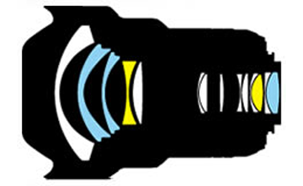
Sample 1: The structure diagram of the Nikon AF-S NIKKOR 14-24mm f/2.8G ED. Nikon’s official material lists it as 14 elements in 11 groups, including 2 ED elements and 3 aspheric elements, and it uses Nano Crystal Coat. Source: Nikon official product page.
This lens is the perfect teaching material for explaining “why an SLR ultra-wide is so complex and irascible.” The angle of view at the 14mm end is breathtakingly wide, but an F-mount SLR must reserve enough back-focal space at the tail for the mirror, so the front of the lens can only be forced to adopt an extremely violent retrofocus approach. In this structure diagram, what is most striking is not the element count at all, but that group of exaggeratedly large front elements and the multiple aspheres interspersed among them: the huge front group is responsible for sheer-force catching the oblique rays of the large field, the aspheres desperately battle barrel distortion, astigmatism, and corner coma, while the ED glass is used to subdue the lateral chromatic aberration that erupts so easily at ultra-wide edges. It wins beautifully, but the cost it pays is blunt enough: huge volume, heavy dead weight, a bulbous protruding front group, and the awkwardness of being almost unable to use conventional filters.
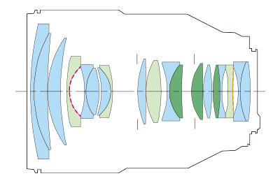
Sample 2: The structure diagram of the Canon RF 28-70mm f/2L USM. Canon Camera Museum material lists it as 19 elements in 13 groups, including a ground asphere, a glass-molded asphere, 1 Super UD element, and 2 UD elements, and it exploits the large diameter and short back-focal distance of the RF mount. Source: Canon Camera Museum.
The RF 28-70mm f/2 is the ultimate sample of “brute-force trading mirrorless degrees of freedom for extreme specs.” Achieving an f/2 aperture at the 70mm end means its entrance-pupil diameter reaches a staggering 35mm, which already approaches the aperture pressure of a genuine 50mm f/1.4 prime; and what is even more terrifying is that it must maintain this monstrous spec across all continuous focal lengths from 28 to 70mm. Canon states bluntly in its official explanation: the RF mount’s huge diameter and extremely short back-focal distance allow extremely thick, large-diameter elements to approach the sensor indefinitely, which provides the physical premise for a leap in edge image quality. The densely packed special elements in the diagram are by no means for showing off, but are extremely arduously coping at once with constant f/2, a wide field of view, the dispersion at the medium-telephoto end, edge aberrations, and the intricate multiple conditions of zooming. The cost of all this materializes into a 95mm filter thread that makes you gasp, a horrifying weight of about 1.43 kg, and a steep price.
Sample 3: The structure diagram of the Canon EF 400mm f/2.8L IS II USM, with the fluorite element and the IS stabilization unit marked. Source: Canon Camera Museum.
A 400mm f/2.8 lens has an entrance-pupil diameter as high as about 143mm, which means the front element’s aperture and material cost will directly punch through the ceiling. In this kind of top-tier professional telephoto cannon, Canon does not stint in installing the most precious fluorite element in the most core part of the front light path, in order to clamp down tight on the most fatal chokepoint of a telephoto lens — axial chromatic aberration and the secondary spectrum; while the IS stabilization group bears no “main imaging” duty at all, but acts as an extremely agile independent moving unit that can be quickly deflected by a high-speed motor to cancel the body’s slight shake. From this diagram, you can clearly read the functional division of labor in a modern telephoto lens: the huge and expensive front elements just greedily devour light and purify color, the light internal moving group handles lightning-fast focusing or stabilization, while the powerful mechanical shell comprehensively serves the speed, absolute reliability, and handholdability under extreme conditions of shooting.
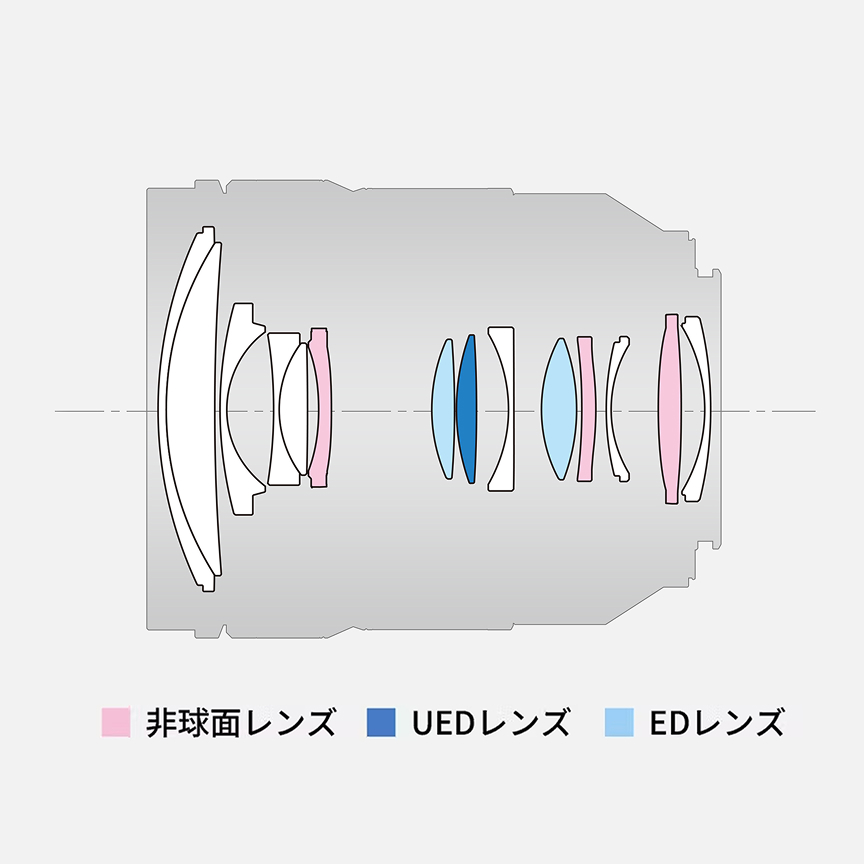
Sample 4: The structure diagram of the LUMIX S 24-60mm f/2.8. Panasonic’s official material lists it as 14 elements in 12 groups, including 3 aspheric elements, 1 UED, and 2 ED; the closest focusing distance is 0.19m (wide end to 30mm) / 0.33m (long end). Source: Panasonic Japan S-E2460.
The most brilliant highlight of this lens is absolutely not “it cuts 10mm off the long end compared to the traditional 24-70,” but that it remarkably and cleverly crams a constant f/2.8 aperture, a wide 24mm angle of view, and strong close-up capability all into a miniaturized shell weighing only about 544g. In the structure diagram, the front group still struggles to support the large field of view and distortion pressure at the wide end, the ED/UED glass arranged in the mid-rear quietly resolves dispersion, and the aspheric elements, while frantically slimming the volume, desperately suppress spherical aberration, distortion, and edge aberrations. It perfectly embodies an extremely pragmatic and clever modern commercial strategy: proactively chopping off a stretch of non-essential telephoto coverage in exchange for a lighter, shorter, handier standard zoom that is extremely friendly to gimbal video shooting.
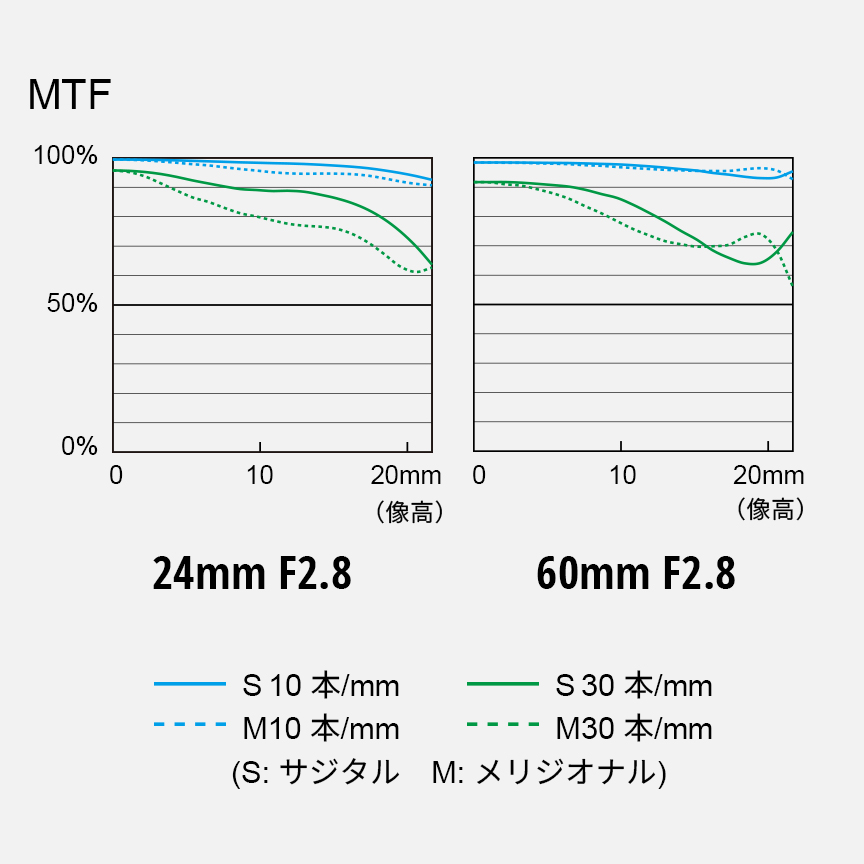
Sample 5: The official MTF chart of the LUMIX S 24-60mm f/2.8. Panasonic notes on the page that, for lenses capable of distortion correction, the MTF horizontal axis is shown as the post-correction center distance. Source: Panasonic Japan S-E2460.
This MTF chart is an excellent cautionary sign: the publicly released MTF curves of modern mirrorless zoom lenses are usually already deeply nested within the system-level context of “lens optics + powerful body/software correction.” Especially at the wide end, in-camera distortion correction forcibly warps the edge pixel-mapping relationship, so you absolutely cannot take it and crudely dunk it side by side against the curves a neighboring manufacturer runs from pure “naked optics.” The truly professional way to read the chart is to return to the purpose itself: does it provide a solid floor of excellent macro contrast and micro detail at both the 24mm and 60mm ends? Do the sagittal (S) and meridional (M) curves split tragically at the frame edge? And what this lens is meant to satisfy — is it the heavy-duty 24-70 professional-workhorse spec, or those creators who crave a lightweight constant f/2.8 and have very high demands for video movement?
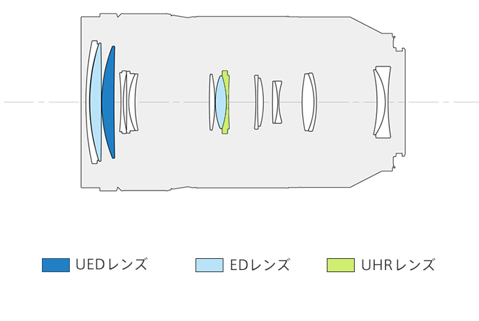
Sample 6: The structure diagram of the LUMIX S 70-300mm f/4.5-5.6 MACRO O.I.S. Panasonic’s official spec is 17 elements in 11 groups, including 2 ED, 1 UED, and 1 UHR; closest focusing distance 0.54m (wide end) / 0.74m (long end), maximum magnification 0.5x. Source: Panasonic Japan S-R70300.
A lens of the 70-300mm focal range is born to answer the ultimate comprehensive question of “how to be long enough, light enough, able to shoot close-ups, and still steady to hold.” It does not have the frightening huge entrance pupil of a professional cannon like the 300/2.8 or 400/2.8, but compromises with a variable and smaller aperture, in exchange for an extremely accessible volume and price. The ED/UED glass in the diagram steadily holds down the chromatic aberration most prone to going off the rails at the long end, while the UHR (high-index glass) handily controls aberrations while greatly shortening the lens structure. The 0.5x maximum magnification grants it formidable half-macro fighting power, but this in turn greatly pressures the engineers: aberrations at close focus absolutely must not collapse, so the precise motion of the focusing group and the aberration-compensation strategy become the key to the whole lens’s success or failure. It is by no means a holy-grail lens challenging the limits of physics, but it is a textbook-level guide to “engineering compromise and balance.”
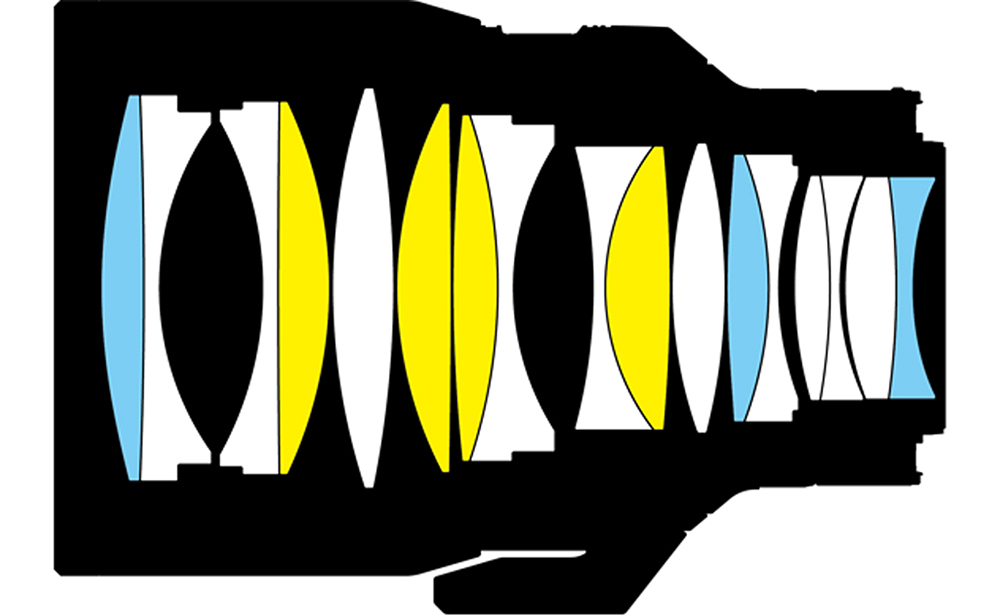
Sample 7: The optical structure diagram of the NIKKOR Z 58mm f/0.95 S Noct. Nikon’s official material lists it as 17 elements in 10 groups, including 4 ED elements and 3 aspheric elements, and it uses Nano Crystal Coat and ARNEO Coat. Source: Nikon Imaging.
If you want to know what “the ultimate brute-force aesthetic” of optical design is, gaze at the Nikon Z 58mm f/0.95 S Noct. Nikon gave it an extremely audacious positioning: an ice-breaking f/0.95 aperture, pure manual focus, and the pursuit at any cost of ultimate point-image reproduction and dominance over night scenes/the night sky. This clearly shows that its objective function dwells on an entirely different plane from all the vulgar 50mm autofocus lenses in the world. An f/0.95 aperture means the entrance-pupil diameter surges to about 61mm, and the cone of light entering the sensor presents an extremely steep angle; at this point, coma, spherical aberration, axial chromatic aberration, vignetting, and focus tolerance are all magnified to hell-level difficulty. The reason it arrogantly abandons autofocus and tolerates a dumbbell-like huge volume is, in essence, sacrificing mobility to the god of optics in exchange for that unmatched optical limit.
Case A: Why Does a 50mm Fast Standard Lens Always Start from the Double Gauss?
Suppose the task you’ve just received is to design a full-frame 50mm f/1.4. First compute the entrance-pupil diameter, which is approximately:
This coldly means an extremely huge array of marginal rays must pour into the lens and be tightly converged onto the image plane within a very short distance. The Double Gauss structure’s near-symmetric skeleton around the stop naturally possesses the magical power to dissolve distortion, coma, and lateral chromatic aberration; the rear negative groups can strongly suppress field curvature and spherical aberration; with this solid foundation, the modern design can then unscrupulously fill in high-index glass, ED materials, high-order aspherics, and a floating-focus group.
This design process can be vividly broken down into:
- First lay the foundation with the Double Gauss and complete the first-order layout: nail down the focal length, stop position, principal planes, and image-circle size.
- Use third-order aberration theory for a preliminary “coarse balancing”: battle distortion, coma, field curvature, and spherical aberration.
- Air-drop in modern degrees of freedom: use aspherics to brute-force suppress residual spherical aberration and coma, and use low-dispersion materials to put out the purple-fringing flames of axial chromatic aberration.
- Implant a floating-focus mechanism: thoroughly seal off the back door where image quality might collapse during close-range shooting.
- Open the full-dimensional comprehensive exam: stew and balance the MTF score, bokeh mysticism, field-curvature flatness, chromatic aberration, distortion, and mass-production tolerances in the same pot over and over.
If the design goal is quietly downgraded to 50mm f/1.8, the entrance-pupil diameter instantly shrinks to 27.8 mm, and the demand for light-gathering area plummets by about 39%. This is exactly why a 50/1.8 “nifty fifty” can always be made extremely small, light, and dirt cheap, yet still output quite capable image quality.
If we look further up, consider the despair-inducing chasm between f/1.4 and f/1.2. The entrance-pupil diameter of a 50mm f/1.2 soars to about 41.7mm, a whole notch larger than f/1.4’s 35.7mm. This leap can certainly buy you intoxicatingly deep bokeh and ultimate composure in low light, but the pressure on axial chromatic aberration, spherical aberration, vignetting, and focusing precision grows explosively. The designer absolutely cannot just take an awl and poke the aperture hole bigger; they must also ensure those extremely manic marginal rays still behave after charging in.
Therefore, a modern 50mm f/1.2 is absolutely no longer the pure Double Gauss of the textbook; it is “the soul of the Double Gauss + a body covered all over in modern god-tier patches”: super-large-diameter front and rear groups, extremely high-precision aspherics, expensive high-index glass, a vast amount of low-dispersion material, complex floating focus, a high-precision motor with violent thrust, and a watertight software-correction matrix. The reason it sells at a sky-high price and weighs like a brick is that the money was all spent on these “patches,” and absolutely not merely for the “boring vanity of a half-stop of aperture.”
Case B: Why Is the 24-70mm f/2.8 Far Harder Than It Looks?
The terror of the 24-70mm f/2.8 lies in this: it is not a single lens at all, but an entire special-forces unit of primes — 24mm, 35mm, 50mm, 70mm, and so on — cruelly and forcibly crammed into an extremely tight barrel; and every focal length must withstand a full-on interrogation across infinity, macro close focus, frame center to dead corners, and light of different wavelengths.
Its typical internal force deployment is as follows:
- Front fixed group: stands guard immovably at the front, deciding the most macroscopic angle of view and intercepting the incident light bundle.
- Variator group: slides wildly inside the barrel, shouldering the core duty of changing the focal length.
- Compensator group: like the variator’s shadow, it pulls back and forth desperately during zooming to ensure the image plane stays nailed to the sensor without drifting.
- Focusing / rear-correction group: responsible for fast focusing, preserving close-up image quality, and polishing the quality of the light that finally reaches the sensor.
If this lens adopts an internal-zoom design, the engineer must also rack their brains to control a constant barrel length and a non-shifting center of gravity; if it must also accommodate demanding video shooting, then breathing, focus drift during zooming, and even the faintest lateral hop of the optical axis will all be deemed unforgivable capital crimes. The so-called “standard zoom” — the water inside is not standard at all; it is downright a hell-level final exam of the integrated fusion of modern optics, precision mechanics, and electronic control.
If we inhumanly dismember the 24-70mm f/2.8 into three endpoints, its difficulty will fill you with despair. At the 24mm wide end, you face the strong pressure of the retrofocus structure, fang-baring barrel distortion, extremely tricky edge incidence angles, and bottomless vignetting; at the 50mm middle, you must hold the extremely demanding balanced image quality of the standard angle of view and absolutely not let it become the performance low point of the whole lens; and advancing to the 70mm long end, you must turn your guns around again to battle axial chromatic aberration, while also tending to bokeh transitions and the dignity of telephoto resolution. Each endpoint is like a beast of an utterly different temperament, yet all must ultimately be tamed within the same barrel, sharing the same mechanical skeleton.
A constant f/2.8 only makes matters worse: it means that even at the 70mm long end, the entrance-pupil diameter must be maintained at about 25mm, which in turn forces the wide end to adopt an even larger and more complex front group to gather light. If a manufacturer maniacally raises the spec to a 28-70mm f/2, the entrance pupil at the 70mm end will reach a terrifying 35mm — already nearly the entrance-pupil scale of a 50mm f/1.4 — yet it must also simultaneously cope with the intricate multi-condition disaster of the zoom system. This is why a lens like the Canon RF 28-70mm f/2L is as big as a bucket and as heavy as an iron discus: it is not an ordinary standard zoom for everyday carry at all, but a desperate, life-risking charge — using the ultimate freedom of the mirrorless system — toward the science-fiction goal of “forcibly merging several fast primes into one.”
Finally, the zoom lens has one more Achilles’ heel that novices most readily overlook but veteran pros hold as sacred: consistency. A professional photographer absolutely cannot tolerate 24mm being one color mysticism and switching to 70mm becoming another color rendering; a video director absolutely cannot stand the focus suddenly getting lost when pushing and pulling the zoom; a news reporter absolutely cannot stand focus hunting back and forth; and a travel blogger absolutely cannot stand it being so heavy it makes you want to chuck it in the trash. The reason the standard zoom is deified as a giant manufacturer’s foundation is that, in design, it has almost no single direction of breakthrough to take — all of its dozens of mutually conflicting metrics must stand on the line of “excellent and passing” all at once.
Case C: Why Are Smartphone Lenses Destined to Go “Computational”?
The physical thickness of a phone camera module has been squeezed to the utmost, and at the same time the individual pixel size of the sensor has shrunk to an outrageous degree. Suppose the aperture is f/1.8 and the wavelength of light is 0.55 µm; by the laws of physics, the Airy-disk diameter at this point is about 2.4 µm; if this phone’s sensor pixels are only around 1 µm, then a fierce hand-to-hand combat has already erupted between the diffraction limit and the sampling rate. Add to this the super-wide field of view, the extremely short focal length, the fully loaded plastic aspheres, machining tolerances, thermal focus drift with temperature, and the CRA matching that must bite the sensor tightly, and trying to achieve “flawlessness” at the level of pure optics is sheer fantasy.
Therefore, the smartphone has unhesitatingly turned fully toward a “system-level computational strategy”:
- At the optical front end: generously allow a certain degree of distortion, vignetting, and even the existence of a field-dependent PSF that deforms severely with position in the frame — as long as the information is not lost.
- At the semiconductor-sensor end: deploy asymmetric microlens offsets and a customized color-filter array to forcibly adapt to those extremely obliquely angled edge rays.
- At the ISP compute hub: unleash thunderous geometric-grid forced correction, brute-force digital brightening of vignetting, AI deep denoising, multi-band sharpening, and multi-frame stacking fusion.
- At the research frontier: even beginning to break with convention, placing the underlying lens curvature prescription and the back-end neural-network image-reconstruction algorithm within the same framework for joint training and optimization.
This is not a regression or degeneration of optical technology, but the formal dimensional ascent of the optical device from an “isolated physical element” into a “computational imaging system.”
Phone photography also offers a highly educational phenomenon: many serious image-quality problems have already been silently smoothed away during the framing-preview stage, before you press the shutter. What you see on screen is by no means the true “naked” image of that plastic lens, but the “cooked” result after distortion reshaping, vignetting removal, denoise bleaching, frantic sharpening, and color mysticism processing. The huge benefit of this approach is that users can always effortlessly obtain a bright, clear photo with excellent bokeh balls; while the cost is that, once the underlying algorithm guesses wrong, those leaf details may be smeared into nauseating oil-painting blobs, the frame edges may be stretched into bizarre shapes, and the texture of night scenes will give off a strong “plastic AI flavor.”
If we elevate our perspective and look at the macro evolution of lens design, the truth of phone photography is by no means “because the lens is too lousy, it can only beg algorithms for rescue,” but “from the first day the project was conceived, it had already carefully calculated outsourcing a vast image-quality budget to algorithms to fulfill.” The optical end need only dutifully provide “sufficiently stable, sufficiently mathematically invertible” incomplete information, and the algorithms will perfectly clean up the rest of the mess. This highly disruptive idea is currently flooding back and profoundly influencing the design philosophy of traditional camera lenses: in-camera DLO (Digital Lens Optimizer), forcibly bound lens-aberration profiles, deep software correction of RAW files, and even end-to-end hardware-software co-design will all irreversibly make future camera lenses more and more like a vast systems-engineering project, rather than just a few pieces of pure glass.
7. Translating Marketing Jargon Ruthlessly Back into Engineering Reality
| Marketing term | The cold engineering meaning | The most common fatal misreading |
|---|---|---|
| Ultimate sharpness | A subjective illusion of sharpness, deeply influenced by MTF, contrast tuning, and post-sharpening algorithms | Naively equating “sharpness” with the lens’s sole optical metric |
| Monstrous resolving power | The limit ability to transfer extremely high spatial frequencies (fine detail) | Staring only at the dead center, completely ignoring edge collapse and close-up shrinkage |
| Chart-topping high MTF | Merely excellent contrast transfer under one particular demanding test condition | Treating it as a cross-brand, cross-focal-length “benchmark score” overall result |
| Earth-shaking large aperture | An extremely huge entrance-pupil area, surging light-gathering, and a wafer-thin depth of field | Completely ignoring the ensuing volume explosion, dead weight, runaway aberrations, and sky-high cost |
| Creamy beautiful bokeh | The mystical result jointly tuned by residual spherical aberration, diaphragm-blade shape, vignetting, and sagittal/meridional consistency | Shallowly assuming “strong background blur (large aperture)” equals “good bokeh texture” |
| Stacking ED/UD/fluorite | A bitter engineering remedy for the material’s dispersion characteristics | Treating the lens as a glass display case, assuming the harder the materials are piled on, the better the image quality must be |
| High-order aspherics | A surface degree of freedom introduced to suppress stubborn aberrations and frantically reduce element count | Deliberately ignoring the rough manufacturing texture, onion-ring bokeh, and high mold costs aspherics bring |
| Internal focus / floating focus | Maintaining aberration balance at different focusing distances through extremely complex internal group motion | Treating it merely as a cosmetic selling point of “fast focusing” or “the lens not extending while focusing” |
| Cinema-grade breathing suppression | Throughout the entire focusing process, the angle of view changes extremely little, with focus transitions and composition rock-steady | Hallucinating that this lens must have higher image quality than others when shooting stills |
| Digital software correction | Proactively conceding, packaging up part of the hard-to-handle distortion, vignetting, and chromatic aberration and throwing it to the body or post-software to solve | Naively assuming all optical disasters can be losslessly fixed by “compute power” |
When you are truly ready to spend hard cash on a lens, the wisest approach is to “reason backward from the scenario,” rather than fantasizing over a spec sheet:
- For portraits: stare at the focal length, whether the working distance is comfortable, whether the bokeh melts away, whether the tonal transition of skin is lush, whether axial chromatic aberration (purple fringing) is jarring, and whether eye-control AF locks on tight.
- For architecture: rigorously check whether the distortion is a weird mustache shape, whether the edge MTF holds up, whether field curvature and astigmatism are flattened, and how much of your precious wide angle of view gets cropped away once distortion correction is turned on.
- For astrophotography: wide open, whether the corner coma and astigmatism stretch the stars into birds, whether the edge point image is solid, and whether vignetting and pupil eclipse leave the corners a patch of dead black.
- For video: examine breathing under a magnifier, listen for whether the focus motor makes noise, whether the aperture ring is stepless and smoothly stepped, whether focus sneaks away while zooming, and the center-of-gravity shift when on a gimbal.
- For macro/product: look only at the maximum magnification, whether the closest working distance blocks the light, the field flatness, whether chromatic aberration is clean, and whether the lens responds well to the in-camera focus-stacking feature.
- For travel: whether the weight will break your neck, whether the focal-length coverage is a jack-of-all-trades, how many stops the stabilization can extend your life by, whether the closest focusing distance can moonlight to shoot some food, whether the anti-flare can be pointed straight at the sun, and whether it is dust- and splash-resistant.
8. A Self-Study Roadmap: From Watching the Show to Seeing the Craft
If we turn this article into a hardcore advanced course, you can systematically train through the following eight modules.
| Module | Core learning goal | The hard bones you must gnaw through | Hands-on practice suggestion |
|---|---|---|---|
| Paraxial-optics foundation | Skillfully computing focal length, principal planes, and magnification | The thin-lens equation, the thick-lens model, the superposition of compound power | Take two lenses and derive the combined system’s focal length and the principal-plane drift |
| Stop and pupils | Thoroughly distinguishing aperture, entrance pupil, exit pupil, f-number, and NA | The stop’s physical position, light-gathering computation, depth-of-field control principles | Compute and compare by hand the real entrance-pupil diameters of a 35/1.4, 50/1.8, and 85/1.2 |
| Aberration-decomposition theory | Developing the venomous eye to “precisely dissect a blurry shot into its specific cause of death” | The five Seidel aberrations, chromatic aberration, wavefront distortion, PSF shape | Hand-draw on paper the ray paths and imaging disasters of spherical aberration, coma, field curvature, and distortion |
| Classic lens-group skeletons | Seeing through the underlying skeleton of a complex modern lens at a glance | Petzval, Triplet, Tessar, Double Gauss, Sonnar, Telephoto, Retrofocus | Among modern lens lineups, find 1 most representative descendant for each classic skeleton |
| Materials and aspherics | Deeply understanding the physical source of modern lenses’ performance surge | ED/UD/fluorite, the anomalous-partial-dispersion curve, the aspheric sag equation | Reason by contrast: without ED glass, what kind of chromatic-aberration disaster would a telephoto lens be |
| Zoom and precision mechanics | Grasping the hellish difficulty of multi-condition optimization | The coupled tracks of the variator and compensator groups, floating focus, internal-focus mechanical structure | Extreme dissection: list in detail all the conflicting constraints a 24-70/2.8 faces at different focal lengths and focusing distances |
| Testing and comprehensive evaluation | Thoroughly quitting the superstition of a single benchmark chart | The connections among PSF, OTF, and MTF, and the test standards for distortion, vignetting, and flare | Grab any manufacturer’s MTF chart and write a report detailing what it “can prove” and what it “deliberately hides” |
| The computational-optics frontier | Touching the boundary of modern optical systems engineering | Sensor CRA matching, ISP intervention, DLO, deconvolution algorithms, end-to-end AI optimization | Analyze in depth a flagship phone’s lens module and explain why “simply blaming phones for relying on software correction is extremely naive” |
9. Conclusion: A Lens Is Never a Perfect Piece of Glass — It’s the Art of “Smart Compromise”
The century-long evolution of the photographic lens is, in essence, a history of optical engineers wresting “more degrees of freedom” from the laws of physics by any means necessary.
In ancient times, a single element could only pitifully rely on changing its shape and stopping down the diaphragm to barely keep aberrations from spinning completely out of control; the Petzval turned fast portraiture from empirical mysticism into precisely computable engineering; the Cooke Triplet, with just three elements, miraculously built a complete underlying framework for aberration correction; the Tessar pushed the efficiency of this framework to a pragmatic peak; the Double Gauss, with its elegant symmetry, firmly ruled the throne of the fast standard lens; the Sonnar, with a do-or-die approach of reducing air interfaces, held the line on high contrast in an era of extremely primitive coatings; the Telephoto and Retrofocus, through near-cheating space-folding of the principal plane, forcibly adapted to the physical dead ends of telephoto and SLR wide-angle; and to this day, zoom, floating groups, aspherics, ED, fluorite, nano-coatings, optical stabilization, and electronically controlled voice-coil motors have already armed the modern lens into an extremely precise opto-mechanical-electronic integrated system; smartphones and frontier research like DeepLens have, without hesitation, pushed the lens headlong into the vast ocean of computational imaging.
So, to truly understand lenses is by no means to recite, like a bookworm, how many ED elements some manufacturer stuffed into a lens, nor is it to glance at an MTF curve’s height and rashly pronounce a death sentence on image quality. True “understanding” is being able, when facing an overwhelming barrage of marketing slogans, to coldly translate them back into cruel physical-constraint conditions: what skeleton does this lens actually rest on? Which aberrations did it pour all its effort into holding down? Just which expensive degrees of freedom did it deploy to buy its current performance? And which costs of compromise did it ever so cunningly hide deep within the weight, price, harsh bokeh, aggressive software correction, collapsed close-up performance, or lottery-like mass-production tolerances?
In lens design, there has never been an isolated and unique “perfect standard answer.” It is more like a philosopher posing a question to the world: in order to finally arrive at that heart-stirring image, exactly which imperfections are worth tolerating and retaining, which imperfections must be eliminated at any cost, and which imperfections can be ever so cleverly passed off to the next link in the system to solve?
Key References
- Petzval lens - Wikipedia
- Filmmakers Academy: What Does a Petzval Lens Do?
- Seidel sum - Britannica
- Abbe sine condition - Wikipedia
- US568052A - Lens patent
- ZEISS: The Planar lens icon
- ZEISS: Lens names Tessar technical article
- Angenieux: Inventions signed Pierre Angenieux
- Canon: RF Lens World - Advantages
- Canon: RF Lens World - Technology
- Canon: Reading and understanding lens MTF charts
- Canon Camera Museum: RF28-70mm F2 L USM
- Canon Camera Museum: EF400mm f/2.8L IS II USM
- Canon Camera Museum: EF 75-300mm IS
- Nikon: AF-S NIKKOR 14-24mm f/2.8G ED
- Nikon: NIKKOR Z 58mm f/0.95 S Noct
- Nikon: Lens glossary
- Nikon: OPTIA wavefront aberration measurement
- Nikon: Extra-low Dispersion Glass
- Panasonic Japan: LUMIX S 24-60mm F2.8 S-E2460
- Panasonic Japan: LUMIX S 24-60mm F2.8 S-E2460 specifications
- Panasonic Japan: LUMIX S 70-300mm F4.5-5.6 MACRO O.I.S. S-R70300
- Panasonic Japan: LUMIX S 70-300mm F4.5-5.6 MACRO O.I.S. S-R70300 specifications
- Sony: Alpha lens technology
- Edmund Optics: Lens iris aperture setting
- Edmund Optics: All about aspheric lenses
- Edmund Optics: Introduction to Modulation Transfer Function
- Schneider Kreuznach: Telecentric lenses
- STMicroelectronics: Lens CRA matching recommendations
- Stanford ISETCam: Optics depth and defocus
- DeepLens - Nature Communications
- DeepLens GitHub
- University of Chinese Academy of Sciences: Modern Optical Design course syllabus